Seen from Space 2020
Massive bushfires in Australia seen from Space
Australia has naturally faced many droughts and bushfires, but conditions have been unusually severe this time. Sometime around September 2019, the bushfires continuously occurred around the state of New South Wales in southeast Australia. The fires had been spreading on a larger scale, and a number of massive fires had merged into a "Mega Fire" that was out of control. The fires are unlikely to end entirely even at the end of January 2020.
Bushfires cause not only personal and economic damages, but also environmental degradation for many animals and discharging carbon dioxide to the atmosphere. There are growing concerns about serious damage to habitats for wild animals including koalas, too. This article introduces the results of diversified analysis on the bushfires by using multi-satellite data.
■ Status of Drought
One of the backgrounds of the forest files is the condition of "drought" especially in the eastern Australia, which has very little rain compared with normal year. JAXA has generated and provided global precipitation distribution data called "Global Satellite Mapping of Precipitation (GSMaP)" using multiple satellite data, such as the Global Precipitation Measurement(GPM) and Global Change Observation Mission-Water "SHIZUKU" (GCOM-W). GSMaP data are available since March 2000 and can be utilized in statistical analysis because it has a long-term data set containing satellite precipitation data with less than twenty years. EORC tried to detect drought happened in Australia by calculating Standardized Precipitation Index (SPI) from GSMaP. SPI is the statistical exponent by which we can evaluate drought only using precipitation amount.
Figure1 (left) shows SPI calculated by GSMaP precipitation amount in a month (December 2019) and Figure1 (right) shows SPI in three months (October-December 2019). Both calculations show the negative value of SPI in most parts of Australia. This means the precipitation amount is less than average. Especially, there are many extreme dry regions including main breadbasket. In the Murray-Darling basin in the east, the SPI value indicates less than -1.5(Severe dryness) or -2.0 (Extreme dryness). This result corresponds to the drought report by The Bureau of Meteorology (Australia) in December 2019.
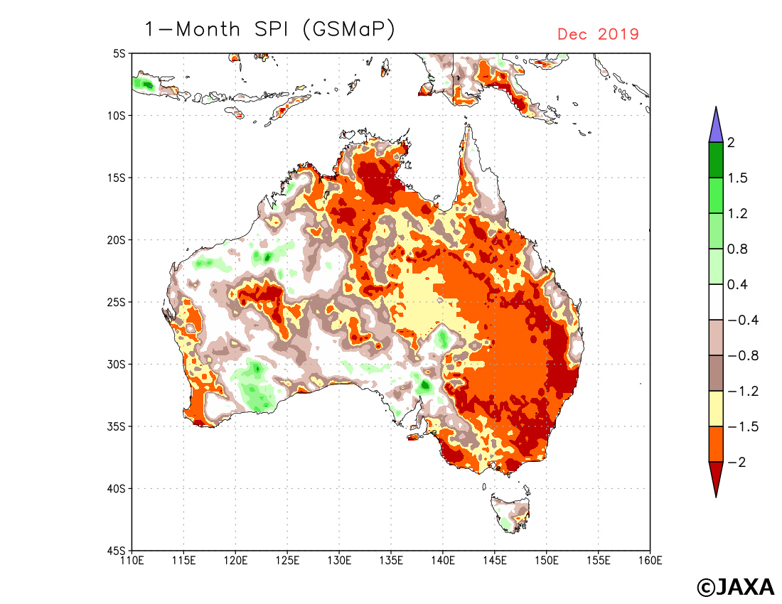
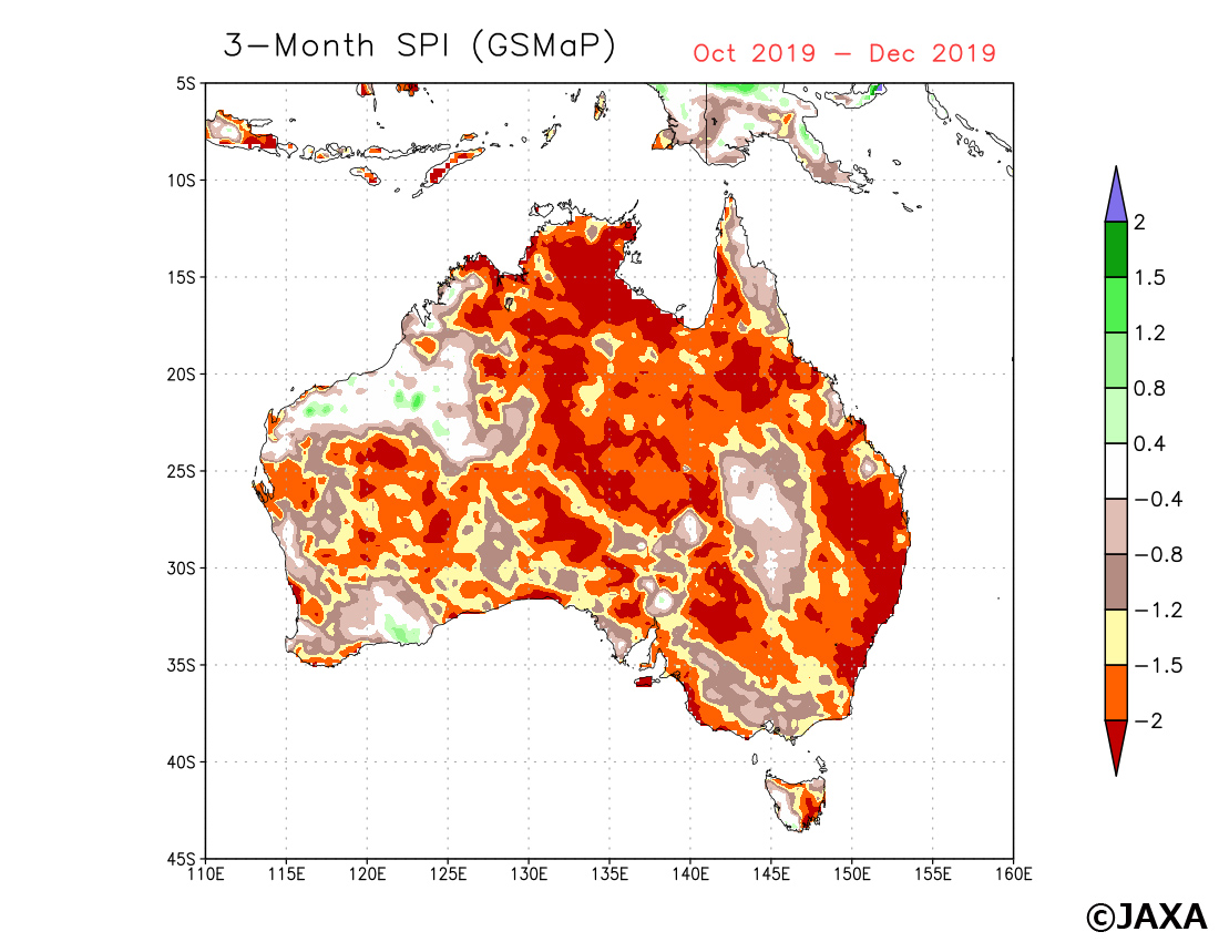
Figure 1 (left) Standardized Precipitation Index (SPI) in Australia calculated by GSMaP precipitation amount in a month (December 2019), (right)SPI calculated by GSMaP precipitation amount in three months (October-December 2019) in a same way. The relations between SPI value, the range of drought and frequency of phenomenon were classified by WMO (2012). In case SPI value becomes "-1.5 to -1.99", it indicates the situation of "Severe dryness" which happens "once in 20 years". In case SPI value becomes less than -2.0, it corresponds "Extreme dryness" which happens "once in 50 years". These condition shows the possibility of severe drought occurrence which leads to a big social impact.
As seen above, the bushfires have occurred frequently on a widespread basis in Australia since last autumn, especially around the state of New South Wales in the southeast with the condition that the eastern area was extremely dry than average year.
■ Status of smoke with fires and aerosol
Figure 2 is the video of RGB composite image every 10 minutes observed by the Advanced Himawari Imager (AHI) onboard Himawari-8 during the term from December 30, 2019 to January 5, 2020. Cloud areas look white and the smoke from fires looks blown. The video shows the smoke has been spreading broadly from fires occurred in the eastern Australia beyond New Zealand. Figure 3 shows the brightness temperature difference of the thermal-infrared channels (difference of brightness temperature between wavelengths of 11µm and 12µm) in the same term and the area. It assumes that this area covered with smoke not dust because the brightness temperature difference does not small with blue color in the areas looks brown in Figure 1 (the difference becomes small in case of the mineral particles).
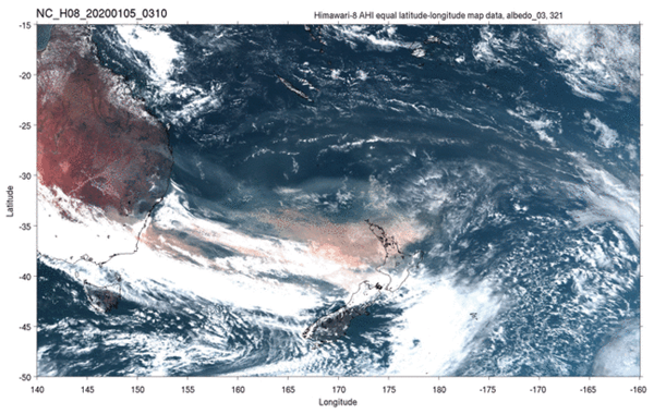
Figure 2 Video with RGB image every 10 minutes captured by Himawari-8 AHI in the area from eastern part of Australia to South Pacific Ocean (December 30, 2019 - January 5, 2020)
Click to play.(Animated GIF format 164MB)
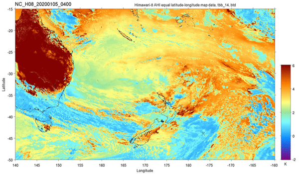
Figure 3 Same as Figure 2. Video image of the brightness temperature difference of the thermal-infrared channels (difference in brightness temperature between wavelengths of 11µm and 12µm)
Click to play.(Animated GIF format 300MB)
The Second-generation GLobal Imager (SGLI) on Global Change Observation Mission -Climate "SHIKISAI" (GCOM-C) can obtain more information compared with the geostationary meteorological satellites. Although its observation frequency is lower, "SHIKISAI" is capable to observe with high spatial and spectral resolution. Figure 4 shows the color image (left column) and the polarized reflectance (right column) observed by "SHIKISAI" on January 1 2020 (Upper line) and January 5 2020 (Bottom line).
When conducting polarization observation from the satellite, the smoke from the fires looks bright with sunlight scatterings (Introduction: Polarization of near ultraviolet observation by "SHIKISAI"). The smoke appeared around Sydney on January 1 and we can find that the polarization reflectance becomes higher near the area. The smoke had been spreading widely and reached around New Zealand on January 5.


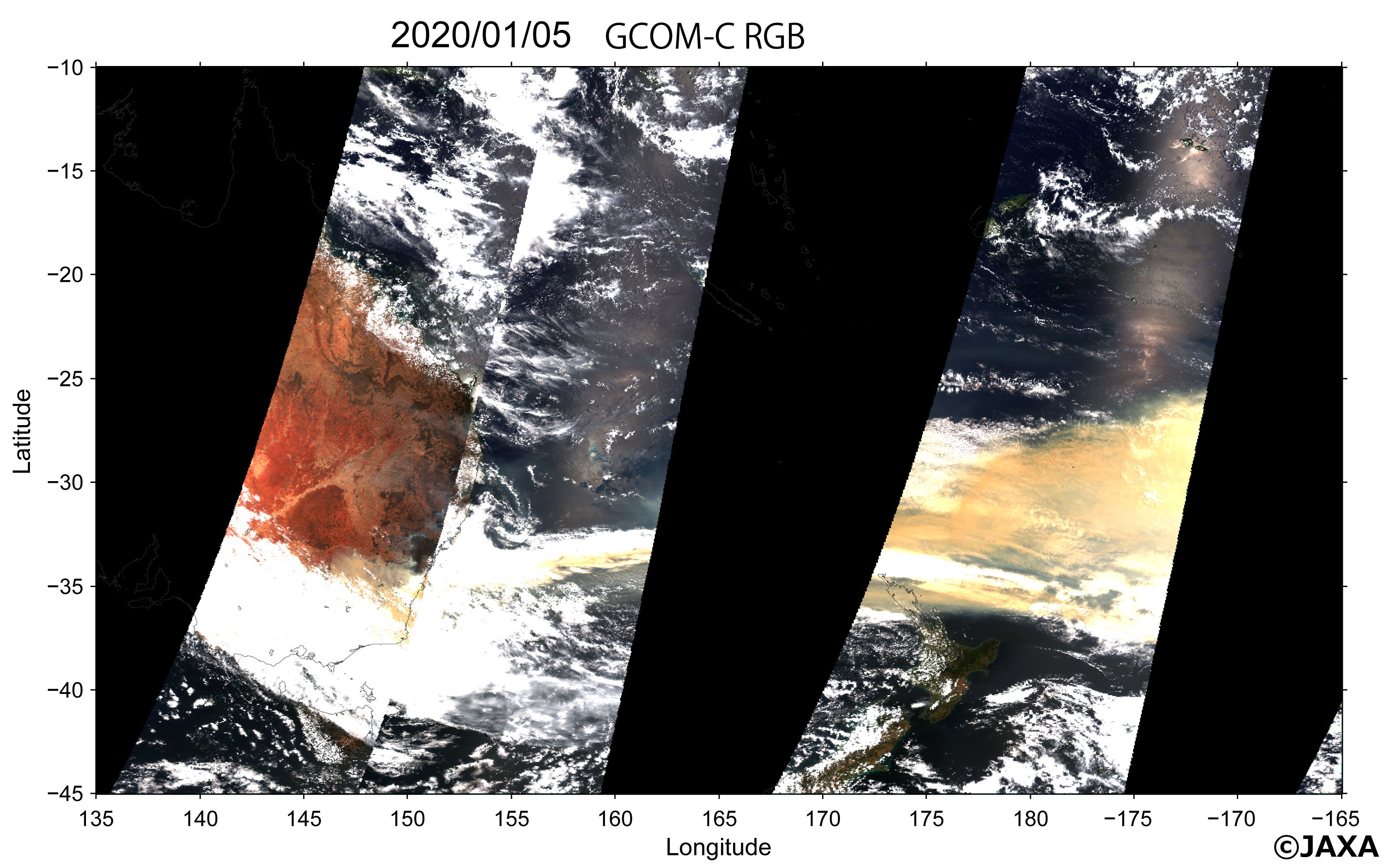
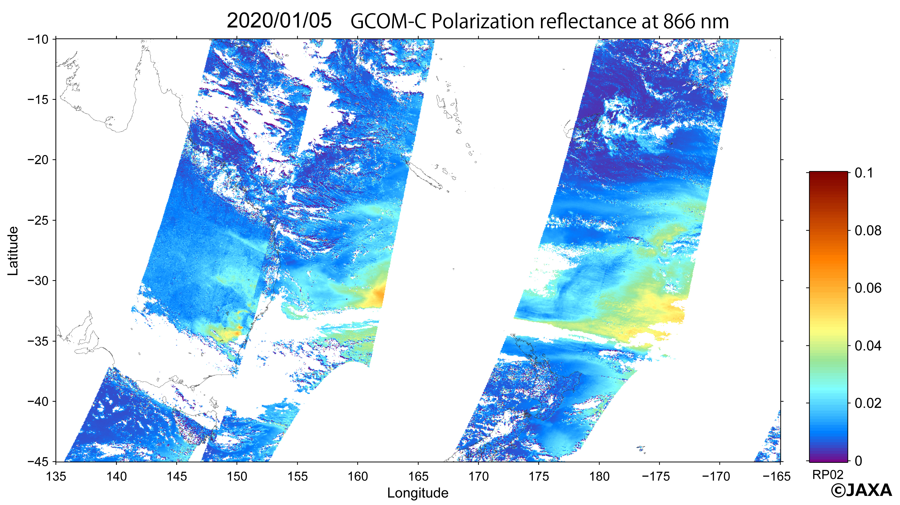
Figure 4 (Upper line) image of descending orbit around Australia observed by "SHIKISAI" on January 1 2020. (Bottom line) image on January 5, 2020. (left column) Color image by "SHIKISAI" (Black area is outside the scope of observation). (right column) polarized reflectance captured by "SHIKISAI" (White area is outside the scope of observation or cloud zone).
JAXA estimates aerosol property by applying coherent algorithm during the observation by Himawari-8 and "SHIKISAI". JAXA conducts joint research for the information regarding aerosol of these satellite observations assimilating into the Model of Aerosol Species IN the Global AtmospheRe (MASINGAR) with Meteorological Research Institute of Japan Meteorological Agency and Kyushu University. Figure 5 shows the video of distribution of aerosol types every hour by this model output during the term from December 30, 2019 to January 5, 2020. The result of this joint research has started to be utilized on Aeolian Dust Information at Japan Meteorological Agency's website since January 29, 2020. (Joint press release on January 24, 2020).
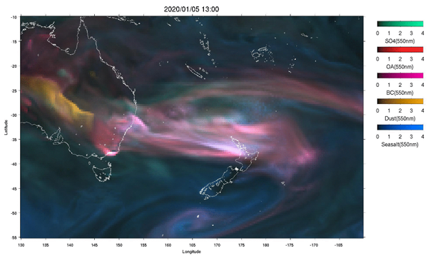
Figure 5 RGB image of aerosol speciation from eastern Australia to South Pacific Ocean during the term from December 30, 2019 to January 5, 2020 by MASINGAR which assimilates Himawari-8 etc. The colors in the image; Green-sulfate, red-organic carbon, purple-black carbon, orange-dust, and blue-sea salt.
Click to play.(Animated GIF format 171MB)
Video of global scale
Daily aerosol by the model of Meteorological Research Institute which assimilates the Himawari aerosol product.
MASINGAR is the Model of Aerosol Species IN the Global AtmospheRe. It conducts assimilation of aerosol optical thickness estimated from Himawari and MODIS. The assimilation system has been developed and operated by Meteorological Research Institute and Kyushu University, and the product is provided by JAXA P-Tree website.
■ Viewing the burnt area
Cloud and Aerosol Imager (CAI) onboard Greenhouse gases Observing SATellite "IBUKI" (GOSAT) has observed the eastern Australia. We cannot detect the smoke from fire on the image of September 1, 2019 but the smoke from massive fires occurred on September 7 seen as two yellow parts. The burned-out area looks black. Then, the smoke seems to disappear when checking the image on November 6, but we can understand that the smoke from the fires has been flown to the Pacific Ocean, the burned-out area has been spreading and the fire spreading has accelerated on November 9. According to the colored image by the difference of November 6 and 9 with a change of these three days, green color shows the burned-out area by fire and the yellow color shows the smoke from swelling fires on November 9.
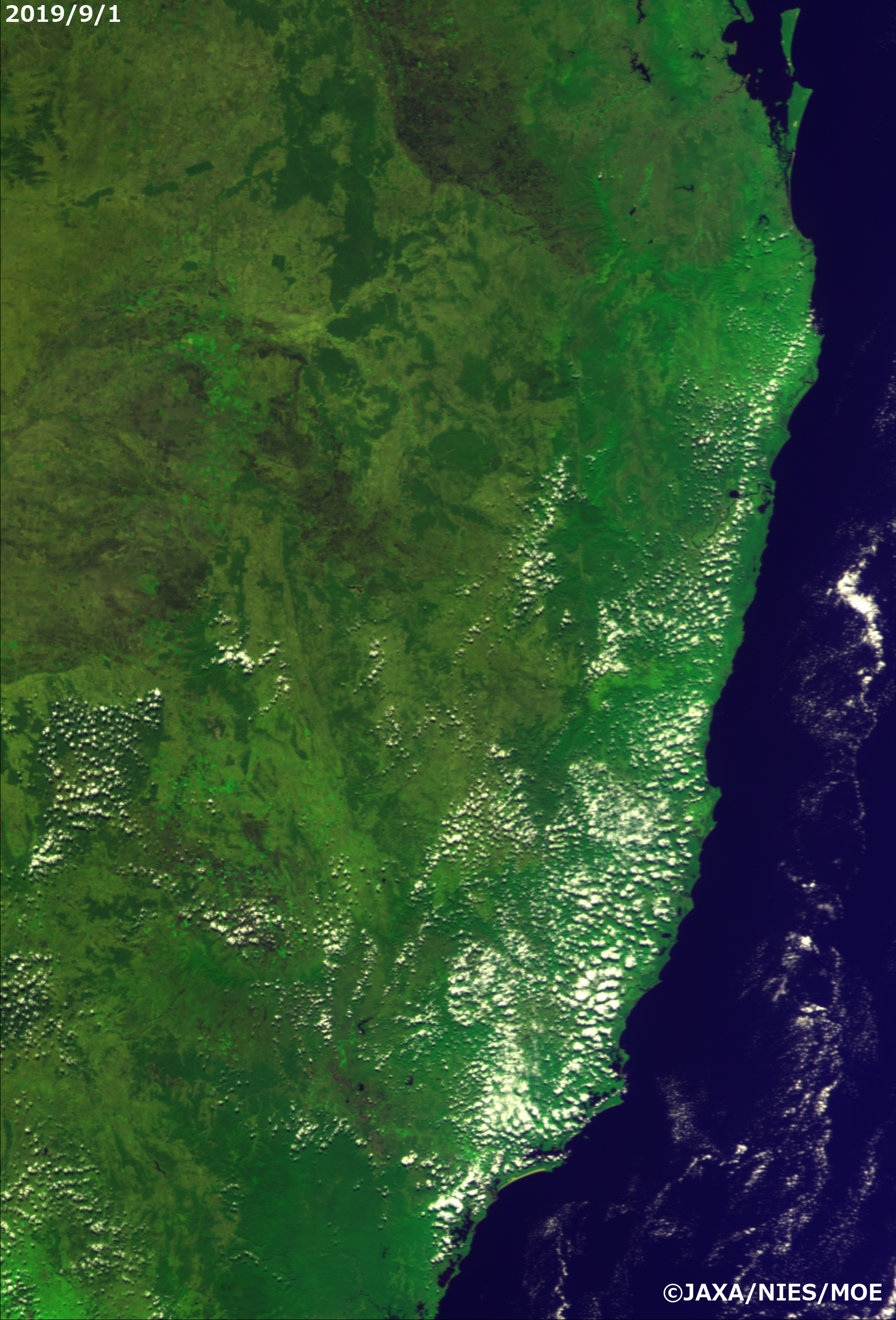

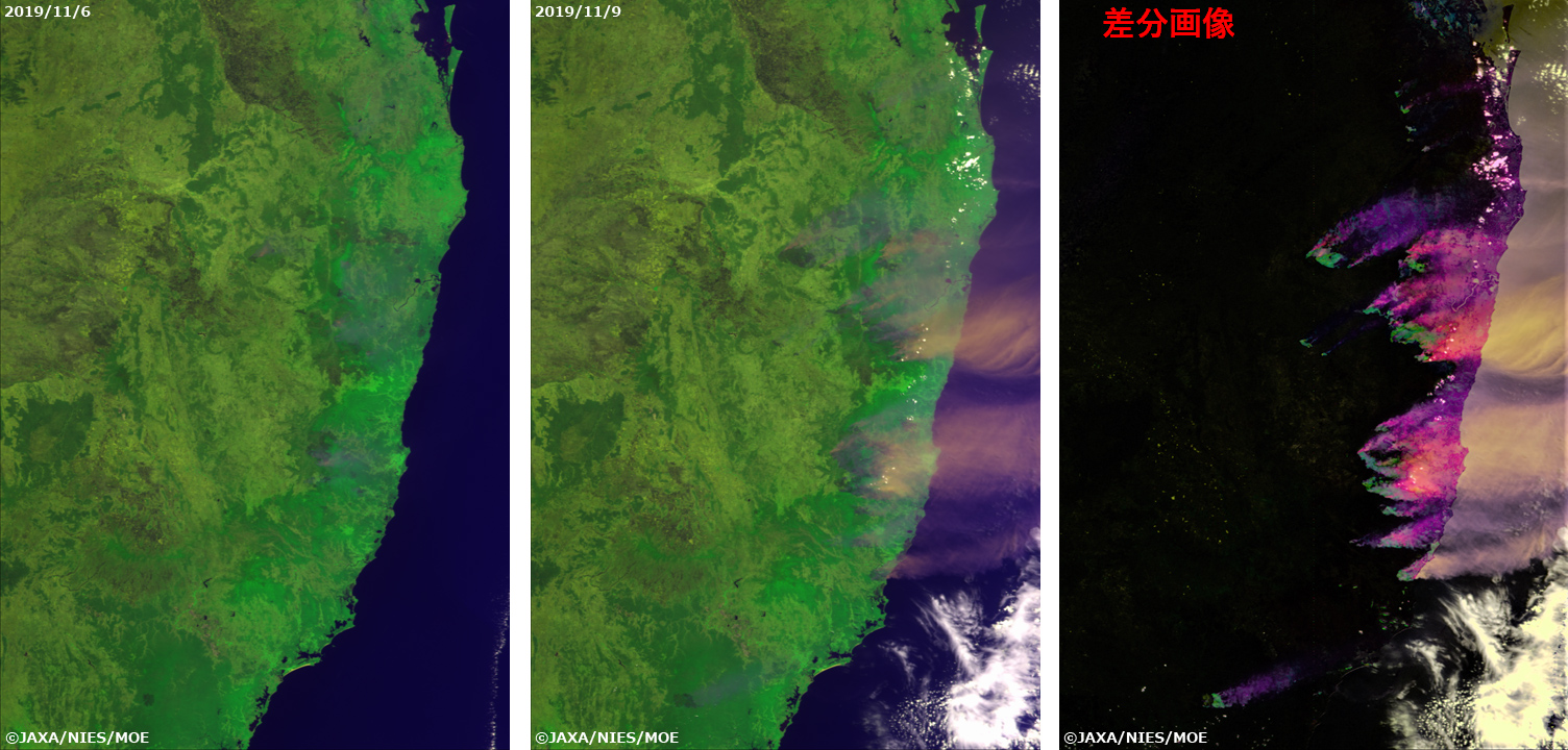
Figure 7 Same as Figure 6. Video of the same area observed every 3 days during November 6 - 21, 2019
■ Viewing the forest area decline
Since "SHIKISAI" and "IBUKI" are using optical sensors, they cannot capture the condition of ground level in case there are clouds over the fire area. On the other hand, the Phased Array type L-band Synthetic Aperture Radar-2 (PALSAR-2) onboard the Advanced Land Observing Satellite-2 "DAICHI-2" (ALOS-2) is capable of observing day and night, and in all weather conditions without the effects of smokes and clouds. JAXA urgently conducted the observation of the bushfires in eastern Australia on January 9, 2020 by ALOS-2/PALSAR-2 and tried to detect the forest area declines.
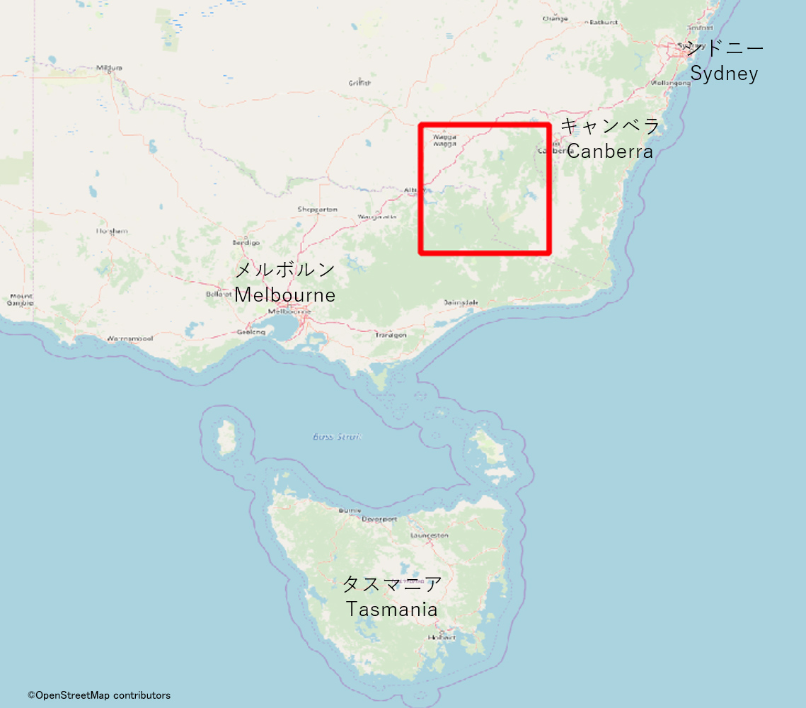
The red square in Figure 8 shows the analyzed range using PALSAR-2 this time. It locates from New South Wales to Victoria in southeast Australia.
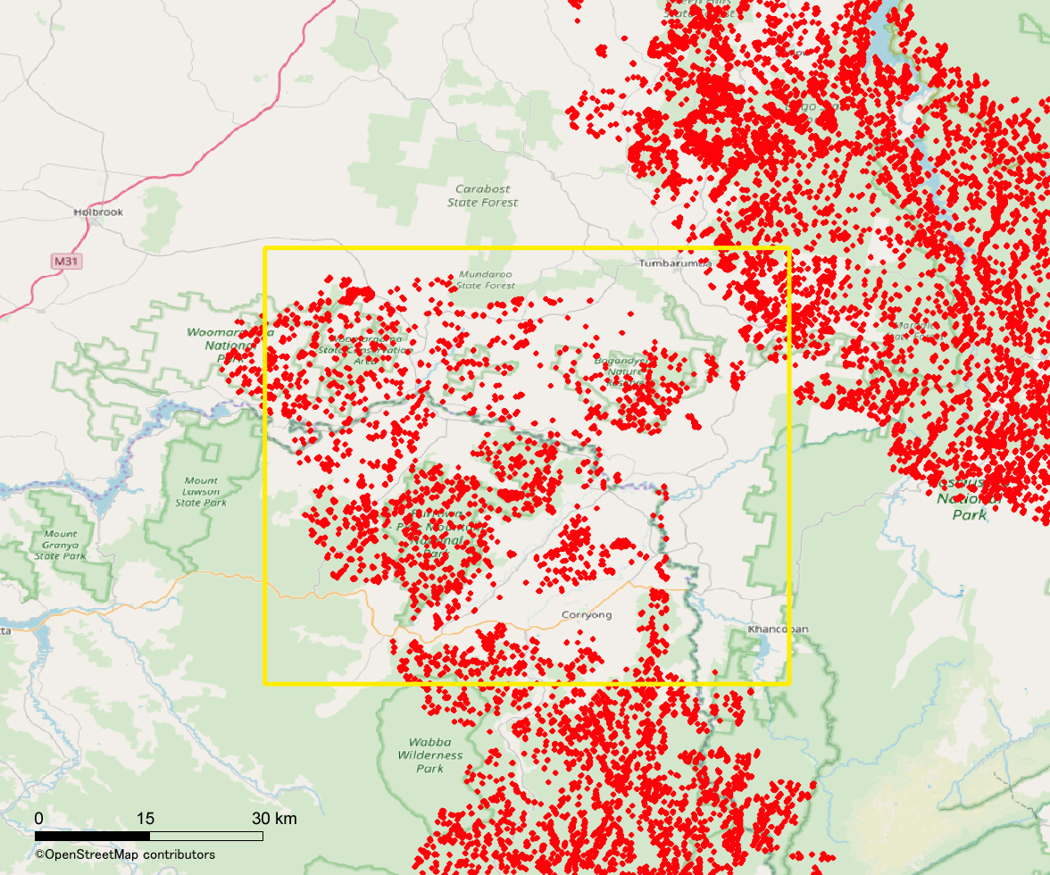
Figure 9 shows the detection result of the forest area declines by overlaying PALSAR-2 images before and after fires with red plots (before image was acquired on January 14, 2016).
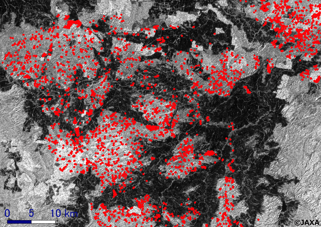
Also, Figure 10 is an example of expansion of the yellow squared frame. The background image is the HV polarized image captured this time. Generally, forest area looks bright in the HV polarization. The forest area declines detected this time as indicated red plots can be found in forest regions. Note that this analysis results may contain the effect of deforestations during 2016-2020.
As described above, we can capture the view of the Earth from various aspects by observing multiple satellites and sensors. JAXA satellites offsets each weak point using each strong observation capabilities such as physical amount, frequency, spatial resolution, cloud transmission and so on.
Explanation of the Images
Figure 1.
| Satellite | Global Precipitation Measurement core observatory(GPM core observatory) Global Change Observation Mission-Water "SHIZUKU"(GCOM-W) |
|---|---|
| Sensor | Global Satellite Mapping of Precipitation(GSMaP) Advanced Microwave Scanning Radiometer 2(AMSR2) |
| Date | December 2019 (Left) October - December 2019 (Right) |
Figure 2,3,5.
| Satellite | Geostationary Meteorological Satellite "Himawari-8" |
|---|---|
| Sensor | Advanced Himawari Imager (AHI) |
| Date | December 30, 2019 - January 5, 2020 |
Figure 4.
| Satellite | Global Change Observation Mission -Climate "SHIKISAI" (GCOM-C) |
|---|---|
| Sensor | Second generation GLobal Imager (SGLI) |
| Date | January 1, 2020 (Upper panels) January 5, 2020 (Lower panels) |
Figure 6 and 7.
| Satellite | Greenhouse gases Observing SATellite "IBUKI" (GOSAT) |
|---|---|
| Sensor | Thermal And Near infrared Sensor for carbon Observation, Cloud and Aerosol Imager(TANSO-CAI) |
| Date | September 1, 2019 and September 7, 2019 (Figure 6, From top left) November 6, 2019 and November 9, 2019 (Figure 6, From bottom left) November 6 - 21, 2019 (Figure 7) |
Figure 10.
| Satellite | Advanced Land Observing Satellite-2 "DAICHI-2" (ALOS-2) |
|---|---|
| Sensor | Phased Array type L-band Synthetic Aperture Radar-2 (PALSAR-2) |
| Date | January 9, 2020 |


