At the IMCET period, enhanced sonde operation by JMA was performed. This
enhanced sonde operation was a part of activity of the GEWEX Asian Monsoon
Experiment (GAME). Using the sonde data set, we tried to get apparent sensible
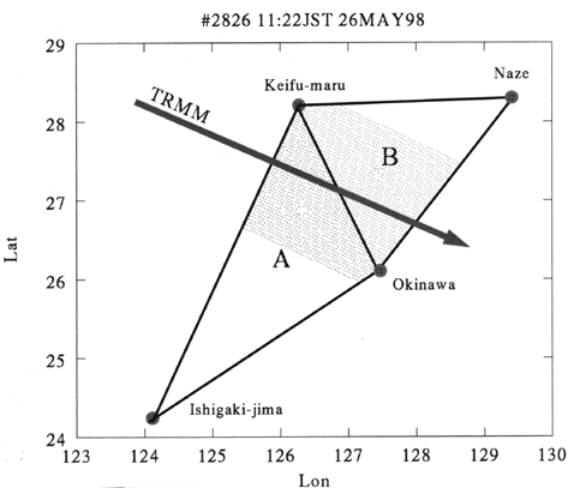
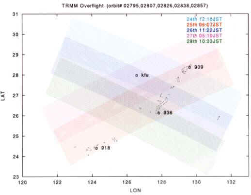
and latent heat budget. Figure 5.1 shows the sonde operation sites related to
IMCET with a PR swath on 26 May. We had 4 sites: Naze, Okinawa, Keifumaru (JMA's
meteorological observation vessel) and Ishigakijima.
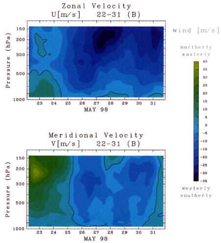
The analyzed period was from 22 May to 31 May. Figure 5.2 shows the zonal and
meridional wind velocity for Region B during this period. Sonde data for three
sites surrounding Region B are averaged. North-Easterly wind was dominant before
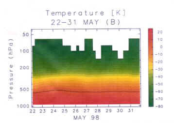
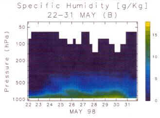
25 May, followed by South-Westerly wind. Figures 5.3 and 5.4 are the temperature
and the specific humidity. After 25 May, lower atmosphere was more humid.
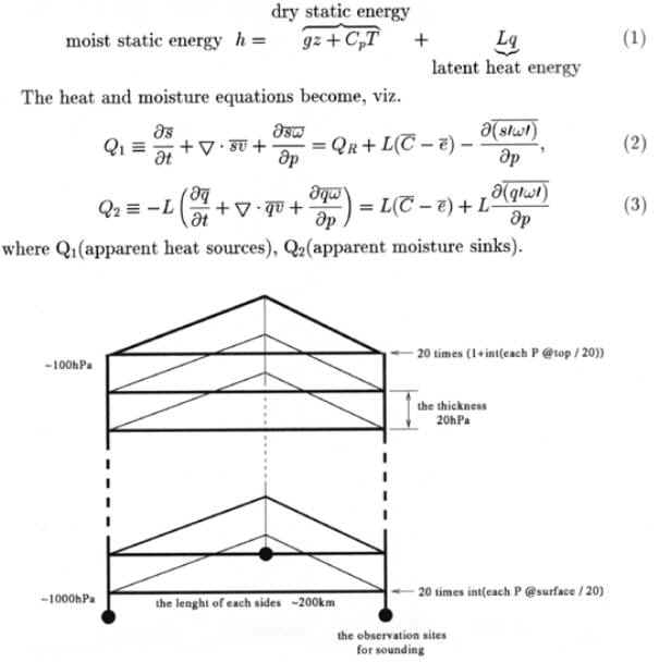
Using three sonde soundings, we calculated the budget for each triangle (A and
B). Figure 5.5 shows the basic formula for the calculation of the diabatic
heating using sonde observations. We sliced the atmosphere into layers of about
20 hPa from near surface (about 1,000 hPa) to up to about 100 hPa. The most
erroneous one is the up/down draft estimation using continuity equation. We
tried to set zero at the lowest level or at the top (usually about 100 hPa where
sonde data is available). Since the former did not give reasonable result, we
mainly used the latter condition. We also tried a linear combination of them.
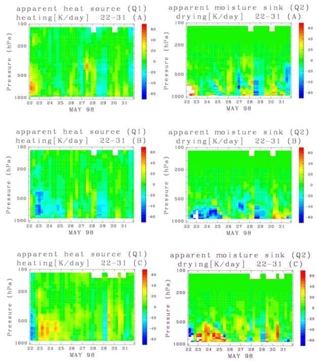
Figure 5.6 shows the result of Q1 and Q2 for each region. Region C is a triangle
one with Minami-Daitojima, Okinawa and Naze).
Estimation of the profile of latent heat release is one of the targets of
TRMM. A very simple algorithm for the estimation is to have a vertical
derivative of the rainrate measured by the PR. The rainrate is vertical water
flux. If all the water condensed from water vapor becomes precipitation. The
vertical derivative of the rainrate become the amount of the condensation if
lateral flux is negligible. The lateral flux may be neglected when we take
sufficiently large area, in other words, make the lateral boundary has no
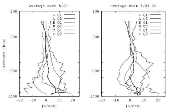
precipitation or cloud. The averaged Q1 and Q2 over the period for each region
(A, B and C) are shown Figure 5.7.
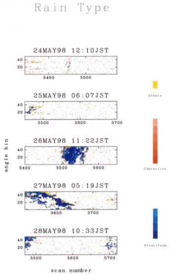
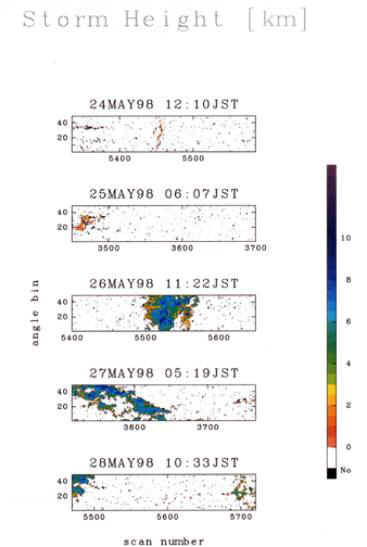
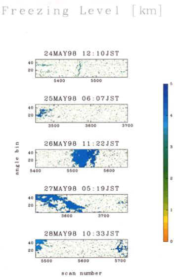
Figure 5.8 is the PR observation for 24 to 28 May. We had only five
overpasses during that period. The precipitation type were mainly stratiform as
shown in Figure 5.9. The storm heights were more than 6 km on 26, 27 and 28 May
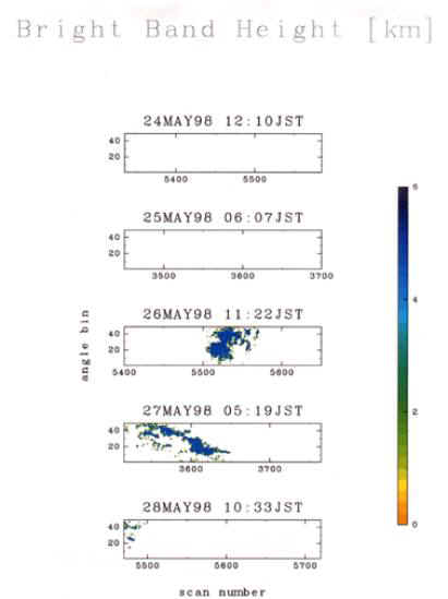
as shown in Figures 5.10 and 5.11. The bright band height and the freezing
levels were about 5 km, which is a typical one during this season (Figures 5.12
and 5.13).
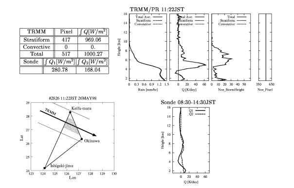
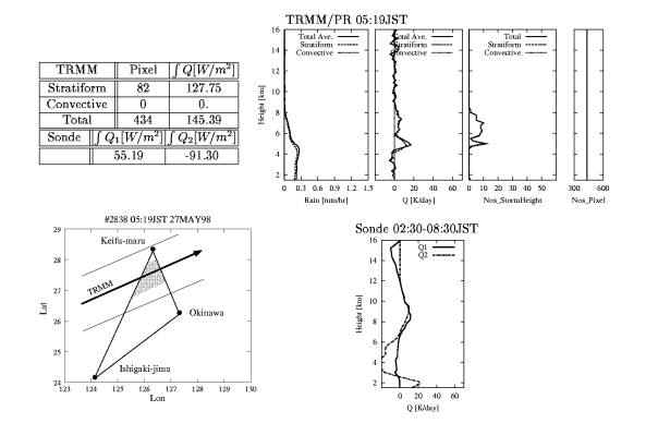
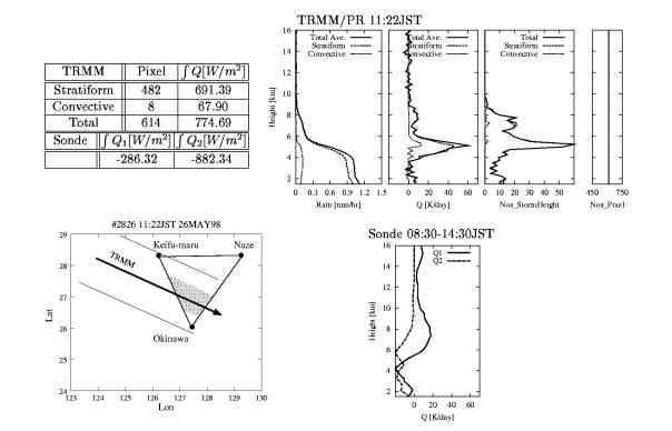
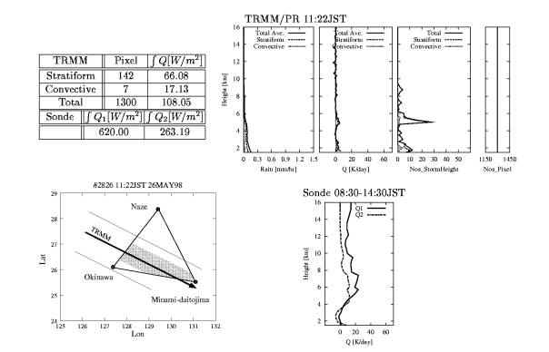
Figures 5.14 (a)-(d) show the vertical rain structure, etc. averaged over the
area (A), (B) or (C). The vertical derivatives are also shown. Since the profile
of rainrate shows the bright band, the vertical derivatives show a positive peak
just above the bright band, and a negative peak just below the bright band.
Though the PR algorithm uses a Z-R relationship for the melting layer, the
bright band is still apparent. This suggests that the PR algorithm should take
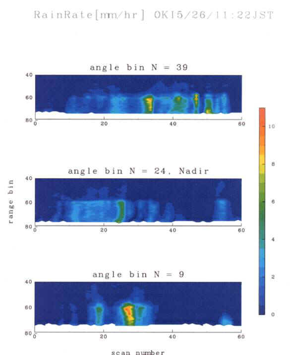
care of the bright band more precisely. The bright band is also appeared in
Figure 5.11, which shows the vertical cross section of precipitation observed by
the PR.
As a summary, the vertical derivative of the precipitation estimated by the
PR has some similarity with the estimation from radio sonde data. There,
however, exist many discrepancies. Once is due to up/down draft estimate from
sonde data. Generally speaking, the rain case we analyses was not so heavy one
and the estimation from sonde data has inevitably much errors. Rain rate
estimation at bright band is also an error cause.
Fig. 5.1 Sonde operation sites related to IMCET with a
PR swath on 26 May.
Fig. 5.3
Temperature for Region B from 22 May to 31 May.
Fig. 5.2
Zonal and meridional wind velocity for Region B from 22 May to 31 May.
Fig. 5.4
Specific humidity for Region B from 22 May to 31 May
Fig. 5.5 The basic formula for the calculation of the
diabatic heating using sonde observations.
Fig. 5.6 The results of Q1 and Q2 for region A (upper),
B (middle) and C (bottom).
Fig. 5.7 The averaged Q1 and Q2 over the period for
each region
Fig. 5.8 TRMM PR observation for 24 to 28 May.
Fig. 5.9
Precipitation type observed by the PR.
Fig. 5.10
Storm heights observed by the PR from 24 to 28 May.
Fig. 5.11 Storm heights observed by the PR on 26 May.
Fig. 5.12
Bright band height observed by the PR from 24 to 28 May.
Fig. 5.13
Freezing levels observed by the PR from 24 to 28 May.
Fig. 5.14 (a) Vertical structure of rain rate, Q1 and
Q2 averaged over the area (A, 26May).
Fig. 5.14 (b) Vertical structure of rain rate, Q1 and
Q2 averaged over the area (A, 27May).
Fig. 5.14 (c) Vertical structure of rain rate, Q1 and
Q2 averaged over the area (B, 26May).
Fig. 5.14 (d) Vertical structure of rain rate, Q1 and
Q2 averaged over the area (C, 26May).