JASMES Tutorial

This tutorial shows how to convert GCOM-C/SGLI (Near-Realtime / Standard) data and VIIRS date in netCDF format provided by JASMES service to GeoTiFF.
We will also show you how to display the created GeoTiFF in QGIS.
In this tutorial, we will create GeoTiFF, which is GCOM-C/SGLI standard data (netCDF) converted to physical quantity.

We have prepared the following two tutorial pages to explain how to convert from netCDF to GeoTiFF.
On this page, we show the method (1) using the Python script.
 (1) How to convert netCDF to GeoTiFF using a sample Python script.(Linux) (this tutorial)
 (2) Convert to GeoTiFF using GDAL commands and parameters.(Windows) (Shikisai Portal FAQ)

Please refer to the following page for details of JASMES user registration. JASMES users can use all data published in JASMES services.
JASMES User Registration JASMES Data Access JASMES Data List

Please use this tutorial as follows for your purposes.

・If you want to convert netCDF data to GeoTiFF
 Execute the sample script according to "1. How to use sample script"

・If you want to know what the sample script does
 See "2. Description of script processing"

・If you want to know how to open GeoTiFF in QGIS for use
 See "3. How to open GeoTiFF with QGIS"

1-1. Sample script download

This is a sample script used in this tutorial. Please download it from the button bellow.

Sample script (GCOM-C/SGLI・VIIRS) Download

1-2. Execution enviroment

The tutorial shows an example of execution under Linux.
The sample scripts use Python3.

The following is the runtime environment and Python libraries used when testing the sample scripts.

1-3. Target data list

To get JASMES data, you need to register as a user here. Please refer to here for how to get data after user registration.
Please see below for data for which sample scripts can be used. Target Data List

1-4. Confirmation of data content

(a) Confirmation using SeaSAS
For information on how to use SeaDAS (available for Windows, Mac, Linux) as a tool to confirm netCDF, please see below. View JASMES SGLI Near-realtime data in SeaDAS
(b) Confirmation using ncdump
In this tutorial, we show how to check the data with the netCDF command ncdump as follows. Execute "ncdump -h" to check the data header information.
As described in "long_name", you can convert the data into physical quantity "DN value stored in netCDF * scale_factor + add_offset".
The information used in the tutorial are the highlighted items.

$ ncdump -h [DIR]/GC1SG1_20230101D01D_J0000_L2SG_CHLAQ_3000.nc
 netcdf GC1SG1_20230101D01D_J0000_L2SG_CHLAQ_3000 {
 dimensions:
	longitude = 10800 ;
	latitude = 10400 ;
	start_time = 1 ;
	end_time = 1 ;

 variables:
	float longitude(longitude) ;
		longitude:long_name = "longitude" ;
		longitude:units = "degree_east" ;
	float latitude(latitude) ;
		latitude:long_name = "latitude" ;
		latitude:units = "degree_south" ;
	double start_time(start_time) ;
		start_time:long_name = "observation start time" ;
		start_time:units = "UTC" ;
		start_time:standard_name = "yyyymmdd.hhmmss" ;
	double end_time(end_time) ;
		end_time:long_name = "observation end time" ;
		end_time:units = "UTC" ;
		end_time:standard_name = "yyyymmdd.hhmmss" ;
 	ushort CHLA(latitude, longitude) ;
		CHLA:long_name = "Chllorophyll-a concentration (CHLA) = DN * scale_factor + add_offset [mg m^-3]" ;
		CHLA:units = "mg m^-3" ;
		CHLA:scale_factor = 0.0016f ;
		CHLA:add_offset = 0.f ;
		CHLA:valid_min = 0 ;
		CHLA:valid_max = 65533 ;
		CHLA:missing_value = 65535 ;
		CHLA:no_observation_DN = 65534 ;
		CHLA:mask_for_statistics = 351 ;
 ...
// global attributes:
		:title = "SGLI equal latitude-longitude Japan data" ;
		:id = "GC1SG1_20230101D01D_J0000_L2SG_CHLAQ_3000.nc" ;
		:date_created = "2023-01-02T05:29:04Z" ;
		:product_version = "3000" ;
		:algorithm_developer = "Japan Aerospace Exploration Agency (JAXA)" ;
		:product_level = "Level-2" ;
		:product_name = "Level-2 Japan product (JASMES)" ;
		:satellite = "Global Change Observation Mission - Climate (GCOM-C)" ;
		:sensor = "Second-generation Global Imager (SGLI)" ;
		:pixel_number = 10800 ;
		:line_number = 10400 ;
		:upper_left_latitude = 49.99875 ;
		:upper_left_longitude = 123.00125 ;
		:upper_right_latitude = 49.99875 ;
		:upper_right_longitude = 149.99875 ;
		:lower_left_longitude = 123.00125 ;
		:lower_left_latitude = 24.00125 ;
		:lower_right_latitude = 24.00125 ;
		:lower_right_longitude = 149.99875 ;
		:grid_interval = 0.0025 ;
		:grid_interval_unit = "deg" ;
		:image_projection = "EQA (sinusoidal equal area) projection from 0-deg longitude" ;

 }

1-5. How to run the sample script

Execute "./Sample_nc2geotiff.py" to convert netCDF to GeoTiFF.
Since the item names may differ depending on the netCDF to be input, please refer to the result of "ncdump -h" and modify it.

$ ./Sample_nc2geotiff.py <Input> <Output> <Product>

Argument 1 Input
 Specify the full path of binary file to be input.

Argument 2 Output
 Specify the name of the GeoTiFF file to be output.
 If only a file name is specified, the output will be in the current directory.

Argument 3 Product
 Specify the product corresponding to the file to be input.please refer to the result of "ncdump -h".

From here, the processes of the sample scripts are explained.

2-1. Reading binary data with Python

Read the netCDF using "netCDF4.Dataset".

# read netCDF4
nc = netCDF4.Dataset(INPUT, 'r')
nc.set_auto_maskandscale(False)

Get the necessary values from the read netCDF.
slope/offset/valid_max are used for physical quantity conversion and apper_left_longitude/upper_left_latitude/grid_interval are used for GeoTiFF output.
The names of the items may differ depending on netCDF, so please modify as necessary. (Differences in capitalization, etc.)

The result of "ncdump -h" is used to obtain information as follows.
・The size of latitude(rows) and longitude(columns) are described in "dimensions", so "nc.dimentions['latutude'].size" is used to obtain them.
・The data to be read is CHLA of variables, which is obtained by "nc.valiables[PRD]" using the PRD described in 1-5.
・slope / offset / valid_max are items in nc.variables[PRD], so they are obtained as "nc.variables[PRD].scale_factor".
・upper_left_longitude / upper_left_latitude / grid_interval are global_attributes, so they are acquired as "nc.upper_left_longitude".

### latitude, longitude
#   SGLI STD, VIIRS
dlat = nc.dimensions['latitude'].size
dlon = nc.dimensions['longitude'].size

#   SGLI NRT
#dlat = nc.dimensions['Latitude'].size
#dlon = nc.dimensions['Longitude'].size

data = nc.variables[PRD]

### max, slope, offset
#   SGLI STD, VIIRS
valid_max = nc.variables[PRD].valid_max
slope     = nc.variables[PRD].scale_factor
offset    = nc.variables[PRD].add_offset

#   SGLI NRT
#valid_max = nc.variables[PRD].Maximum_valid_DN
#slope     = nc.variables[PRD].scale_factor
#offset    = nc.variables[PRD].add_offset

### grid_interval
#   SGLI STD, VIIRS
grid_interval = nc.grid_interval

#   SGLI NRT
#grid_interval = 0.0025

### upper_left (pixel center -> top left corner of the pixel)
#   SGLI STD, VIIRS
upper_left_longitude = nc.upper_left_longitude - (grid_interval * 0.5)
upper_left_latitude  = nc.upper_left_latitude + (grid_interval * 0.5)

#   SGLI NRT
#upper_left_longitude = nc.Upper_left_longitude
#upper_left_latitude  = nc.Upper_left_latitude


# pixel size
dx = grid_interval
dy = grid_interval*-1

2-2. Convert to physical quantities using slope and offset values with Python

"DN * SLOPE + OFFSET" is converted to a physical quantity and stored in an array(data type is Float).
Values greater than valid_max are replaced with nan, since they are "no_observation_DN", "missing_value", etc.

# value = DN * slope + offset
val = data*slope+offset
otemp      = np.zeros((dlat,dlon),dtype=np.float32)
otemp[:,:] = val[:,:]
otemp[data>valid_max] = np.nan
otemp = otemp.astype(np.float32)

2-3. Output GeoTiFF with Python (GDAL library)

The array is output in GeoTiFF format using Python's GDAL library.
Create a GDAL driver that creates GeoTiFF.
・driver.Create(output, cols, rows, band, data type)

# GeoTiFF
driver = gdal.GetDriverByName('GTiff')

# outputfile, cols, rows, band num, data type
cols      = otemp.shape[1]
rows      = otemp.shape[0]
outRaster = driver.Create(OUTPUT, cols, rows, 1, gdal.GDT_Float32)

SetGeoTransform with the coordinate values.
・outRaster.SetGeoTransform((upper left longitude, pixel size(x), rotate, upper left latitude, rotate, pixel size(y)))

# upper_left_longitude, pixel size(x), rotate, upper_left_latitude, rotate, pixel size(y)
outRaster.SetGeoTransform((upper_left_longitude, dx, 0, upper_left_latitude, 0, dy))

Specify the band.

# band
outband = outRaster.GetRasterBand(1)
outband.WriteArray(otemp)

The projection method is set to EPSG:4326.

# EPSG
outRasterSRS = osr.SpatialReference()
outRasterSRS.ImportFromEPSG(4326)
outRaster.SetProjection(outRasterSRS.ExportToWkt())

Export to file to output GeoTiFF.

outband.FlushCache()
outRaster = None

print("### END output : "+OUTPUT+" ###")
sys.exit(0)

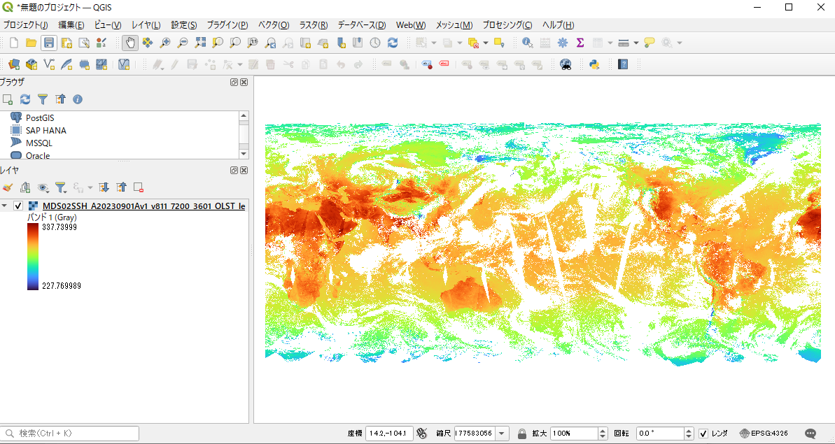
The GeoTiFF created in this tutorial can be opened directly in QGIS, a free GIS software, for viewing, editing, and analyzing data.
Please refer to the following QGIS usage instruction if necessary.

・Display of Chlorophyll-a Concentration (QGIS) (Shikisai Portal)
Please refer to the logarithmic scale (QGIS) if necessary, as the logarithmic scale may be easier to read in some cases, such as CHLA.
Display of Chlorophyll-a Concentration (QGIS) (Shikisai Portal)