EORC / OCTS CAL/VAL group

masanobu shimada

ver. 0 Feb. 5 1998

ver. 1 Feb. 9 1998

ver. 1.1 Feb. 10 1998

Members

OCTS team (NASDA staff)

Hiroshi Kawamura (Leader) Kamu@ocean.caos.tohoku.ac.jp

Masanobu Shimada (Subleader 1) shimada@eorc.nasda.go.jp

Yasuhisa Nakamura (Subleader 2) nakamura@eorc.nasda.go.jp

Hiromi Oaku (Calibration Group Leader) oaku@eorc.nasda.go.jp

Hiroyuki Oguma (Application Group Leader) oguma@eorc.nasda.go.jp

Yasushi Mitomi (Algorithm Group Leader) mitomi@eorc.nasda.go.jp

Akira Mukaida (Validation Group Leader) mukaida@restec.or.jp

Hiroshi Murakami (Application Group Leader) murakami@eorc.nasda.go.jp

Supporting Scientists

Hajime Fukushima (Tokai University)

Ken Furuya (University of Tokyo)

Yoshiaki Honda (Chiba University)

Joji Ishizaka (National Institute for Resources and Environment)

Motoaki Kishino (Institute of Physical and Chemical Research)

Satuki Matusmura (National research institute for far Seas Fineries)

Masao Moriyama (Nagasaki University)

Teruyuki Nakajima (Tokyo University)

Futoki Sakaida (Kobe University of Mercantile Marine)

Sei-ichi saito (Hokkaido University)

Toshiro Saino (Nagoya University)

Yasuhiro Senga (Tokai University)

Sumio Tannba (Iwate University)

In this document, we present the calibration and validation results of the OCTS version 3 products, which are mainly composed of the chlorophyll-a concentration (CHL-a), the normalized water leaving radiance (nLw), and the sea-surface temperature (SST). Calibrating OCTS is to characterize the inter-detector sensitivity, dark current property, and absolute sensitivity using internal and external calibration sources (i.e., AVIRIS underflights). Validation of OCTS tunes the atmospheric correction equation by the vicarious method which uses the in-situ measurement of nLw and the atmosphere, and then, compares the estimated CHL-a and the in-situ data. It tunes the SST retrieval equation. We acquired 17 in-situ data for CHL-a, 11 data for nLw, and 225 for SST. We selected the vicarious calibration coefficients which minimize the residuals for CHL-a within 68% and nLw at 128 % (band 4) to 94 % (band 2). SST was also verified as less than 0.70 K. Geometric accuracy was improved to around 1.3 km. Stripes in the Ocean Color products and the SST products were reduced much more than in previous products.

Appendix also introduces a method for radiometrically converting from the previous version to the version three products.

1. MAIN CHANGES IN VERSION 3 SOFTWARE

1.1 Atmospheric Correction Method

An OCTS-type atmospheric correction algorithm was adopted as in the version 2 software. Several bugs were fixed, and the processing stability was improved. The aerosol selection scheme was improved for quicker convergence.

1.2 Vicarious Calibration and Validation

The calibration coefficients were determined in the vicarious approach using the in-situ data simultaneously acquired during the OCTS passages. Those data were the aerosol type, optical thickness, nLw, CHL-a, etc. A total of 17 CHL-as and 11 nLws were screened as the errorless measurements that were acquired as simultaneously as OCTS observation. Calibrations using the internal lamps and AVIRIS underflight data were conducted. However, this version does not adopt the calibration coefficients derived by those results. The OCTS CHL-a data were compared with the in-situ data.

1.3 Stripes

The stripe elimination function was enhanced significantly compared to the previous version software. This function was modified to enable the detector normalization coefficients dependent on the radiance. (This means we assume nonlinearity in the sensitivity) These calibration coefficients were calculated using the uniform and the various intensity areas. Weak stripes, however, still remain in the larger scanning area. SST stripes were reduced by applying detector normalization coefficients measured from the uniform ocean area. These improvements also removed the stripes in the global products.

1.4 Geometric Location Accuracy

Geometric location accuracy was improved to an error of around 1 km by determining the three offsets in pitch, roll, and yaw so as to minimize the least square error between OCTS pixel location and the ground-control points. Ground-control points were selected from the Japan islands. Global error assessment is a concern as it is in other products.

1.5 Registration

Registration data is originally provided from the ground measurement at the factory. The land products such as the vegetation index require accuracy. Trial-and-error parameter modification improved the registration accuracy slightly.

1.6 Flag Information

Flag information was tuned more confidently than before. The updated flags are the near cloud, land mask, absorptive aerosol flag, identification of the cocolisophere, etc. Land mask information was blocked to enable viewing the ocean color and SST information in the lakes, inland seas, and ponds.

1.7 Cloud Screening

The cloud screening process was improved to exclude suspicious clouds.

1.8 Binned Products

Image quality of the binned products was improved very much.

2.1 Principle

2.1.1 Algorithm

The equations governing the responses among the solar irradiance, atmosphere, ocean system, and sensor characteristics are given below:

A. OCTS digital number - input radiance

The relationship between the OCTS measurements (digital number (DN)) and the input radiance is modeled by:

(1)

where Lti,j is the input radiance to the ith detector of jth band of OCTS (mW/str/cm2/mm); DNi,j, the digital number; Oi,j, the offset of OCTS sensor which is measured in the night time; ai,j, the detector normalization coefficients (relative calibration coefficients to the reference detector whose detector number is five); Gi=5,j, the absolute gain of the i = 5th detector; and Fdata, a reflection property of the scanning mirror which changes as the function of the tilt angle. Fdata measures i.e., 0.974 for band 1 at tilt angle of 20 degrees. Exact expression of Fdata is given in Appendix 3.

B. Water leaving radiance - input radiance

The input radiance to the OCTS can be expressed by the following equations

(2)

(3)

where is the re-calculated radiance so as to satisfy Eq. (2); Lmoli,j, the molecular radiance; Lmai,j, the radiance from the interaction between the molecule and the aerosol; Lai,j, the aerosol radiance; ti,j, the transmittance; and Lwi,j, the water-leaving radiance containing information on the water contents, such as the CHL-a, pigment, k-490, etc. pr is the atmospheric pressure; ta, the optical thickness; oz, the ozone quantity; and OC, the oceanic materials (i.e., chlorophyll and pigments). ej and fj are the vicarious calibration factors (or algorithm tuning factors) to convert Lt to . Here, the first three terms on the right side of (2) are calculated numerically.

This model can work for ten different aerosol types to describe the atmospheric radiation properties in any ocean area (Table 1). More detailed information can be provided by Nakajima et. al.[2] and Fukushima et. al.[4][6][7]

Table 1 Aerosol models installed in OCTS software

Model number Aerosol type Humidity

1 Oceanic 50

2 Oceanic 80

3 Oceanic 90

4 Coastal 50

5 Coastal 80

6 Coastal 90

7 Stratospheric 50

8 Stratospheric 80

9 Stratospheric 99

10 Absorptive

C. Ocean products - water leaving radiance

The relationship between the oceanic materials and the water leaving radiance is empirically expressed by:

(4)

The empirical models adopted for the OCTS data processing subsystem can be found in Kishino et. al.[3].

2.1.2 Definition of the terms

Before the description of the report, we define the terms on calibration and validation. The process flow of these works for ocean color is shown in Fig. 1. Same process flow is valid for sea surface temperature. Calibration is defined to determine the accurate conversion equation from DN to the input radiance (Lt) at the sensor input. Validation contains two processes: first, the algorithm tuning (vicarious calibration) that adjusts the given radiance so as to meet with Eq. (2), and second, the evaluation of the estimated values.

Fig. 1 Overview of the process flow for ocean color case.

2.2 Calibration

2.2.1 Radiometric calibration

A Absolute Calibration

Three data sources were used for calibrating the OCTS measured input radiance. They are the preflight calibration data, optical lamp data, and AVIRIS underflights of OCTS. Appendix 1 summarizes the process flow of the radiometric calibration.

(1) Preflight calibration data The preflight calibration data acquired at the factory were to relate the input radiance (Lt) (mW/str/m2/um) and the digital number (DN) for each detector and each band. The measurement data were obtained by using the integration sphere [1].

(2) Optical lamp data The two calibration lamps were used every 42 days or so, and the data were evaluated in terms of stability, power loss, and the usablity for the calibration sources. The lamp data were assumed as almost constant over eight months or slightly loosing sensitivity. Those data were used to evaluate the radiometric stability.

(3) AVIRIS data Four AVIRIS underflights of the OCTS were conducted off California, USA, on Nov. 7, 1996, and Feb. 28, March 4, and May 20, 1997. The best possible co-registered data were used for evaluating the OCTS stability and its absolute value determination. Fig 1b shows the direct comparison of AVIRIS and OCTS data.

Although these three measurements (plus the vicarious calibration method) are compared, none of the two methods match (Fig. 2a shows the across band sensitivity differences for four different calibration signal sources). We could not conclude which data sources should be relied on. We will therefore continue using the gains Gi=5,j from preflight calibration coefficients in version 3. Offsets of each detector and channel are determined by evaluating the nighttime data. Those data, Oi,j and Gi=5,j, are shown in Tables I and IIs (II-1, II-2, II-3, and II-4). For more detailed information, refer to [5].

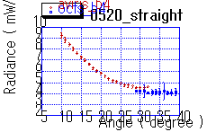
a) b)

Fig. 2 Comparison of calibration coefficients (after H. Oaku)

B Relative calibration - detector normalization

We performed relative calibration of the 80 detectors at visible and infrared bands. If the sensitivities of all the detectors in a band were determined correctly, the image must not suffer from the stripes. However, many stripes were visible in images when we applied the Gi,j (preflight data) or the lamp data. We statistically evaluated the interband-sensitivity variations over 62 different targets on the Earth surface collected from ocean and land, different scan angles, and different tilt angles. Based on this, we made the following interband sensitivity model as a function of the input radiance:

(5)

(5-1)

where ai,j is the detector normalization coefficient for the ith detector of jth band; bi,j, the slope of the ijth detector; Ltempi,j, each detector's input radiance converted by using the gain of the fifth detector and each detector's offset; ci,j, the offset; LCi,j, the criteria by which a different normalization curve is selected. The detector normalization coefficients are given in Tables III, IV, and V. The sample relationship between the ai,j and the input radiance for the seventh detector of bands 6 and 8 is shown in Fig. 3.

Note that the above detector normalization coefficients were determined by using the ocean-normal data and land normal data, then, the images in the other gains may be corrected slightly different.

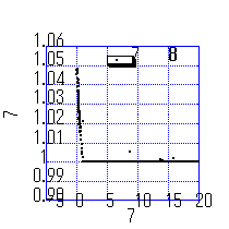
Fig. 3 Detector normalization coefficients aij. a) 7 th detector of band 6; b) 7 th detector of band 8.

2.2.2 Geometric calibration

1) Offset of the attitude values

The geometric accuracies of the OCTS data products are listed in Table 2. Roughly, these values are within 1.31 km. This accuracy was attained by tuning the three components for the alignments between the OCTS and the satellite base plate, and three alignments in the OCTS scanning mirror so as to minimize the least square error of estimated ground points and the measured ground control points. In total 187 ground control points were measured[8].

Table 2 Geometric accuracy improvement by tuning the sensor alignment (km)

Average Standard deviation

Total Cross Along Total Cross Along

Error average 0.15 0.017 1.31 1.03 0.81

Note 187 ground control points were sued for this tuning.

2) Registration parameters

The band-to-band registration is a key parameter for generating satisfactory products for land applications. The complexity of the detector alignment over twelve bands makes it difficult to achieve perfect detector co-registration. The terrain height also makes the co-registration difficult.

Table 3 Accuracy improvement by registration parameter

TBD TBD

2.3 Validation

2.3.1 Algorithm tuning (Vicarious calibration)

Vicarious calibration was conducted using (2) and the in-situ data, such as nLw, aerosol quantities, and the atmospheric properties. The complete datasets for determining the calibration coefficients are very limited. The good datasets were acquired in the CALCOFI experiments off California on November 1, 1997. The vicarious calibration coefficients were selected through the competitive works. Using the truth datasets which contain 11 data measurements, six vicarious calibration coefficients were proposed from several researchers (three from NASDA, two from Tokyo University, and one from Tokai University). An analysis of the difference between the estimated CHL-a and the true CHL-a determined the final calibration coefficients. This conversion is summarized as follows:

(6)

where fj and ej are the tuning coefficients determined for each band.

2.3.2 Evaluation

We collected the in-situ data of CHL-a and nLw world widely in collaboration with national and international agencies and institutes. Out of more than thousands collected in-situ data, those data that were acquired almost simultaneously with OCTS under the cloud free condition were screened. There are 17 CHL-a and 11 water-leaving radiance. Fig. 4-a) shows the scatterogram for the estimated CHL-a and in-situ CHL-a and Fig. 4-b) shows that for the water leaving radiance at band 1. Table 4 summarizes the error statistics. We confirmed the relative error of the CHL-a to be 68% and the water-leaving radiance to be 94 to 128 %. The standard deviation of the error at band 5 exceeds 400%. This may requires the improvement of the calibration accuracy.

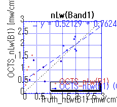
Fig. 4 Error distribution a), the truth CHL-a and estimated CHL-a; b), water leaving radiance.(after Y. Mitomi)

Table 4 Accuracy of the CHL-a and nLw

Items Accuracy (%)

nLw1 96

nLw2 94

nLw3 112

nLw4 129

nLw5 417

CHL-a 68

2.4 Discussion

We acquired as many in-situ data measurements as possible after the satellite launch. During eight months operation from Nov. 1996 to June 1997, we collected 1236 measurements for CHL-a, and 338 for water-leaving radiance. However, the usable data sets were limited due to different time scales, locations, or cloud coverage to about ten for both types of data. This shows that acquisition of the best possible matched data sets is extremely difficult. The success ratio is only 1% (ten divided by one thousand).

3.1 Calibration

Calibration is the validated transformation of the Digital Number to the integrated radiance over the filter characteristics. The unit of the converted value is mW/str/m2.

(7)

where L0i,j is the integrated radiance over each band; Voi,j, the observed voltage; VIi,j, the voltage to the black body; fo, constants; and Og, constants. was measured on-ground and the contents are shown in Table XI.

3.1.1 Absolute calibration

This has not been completed yet. We are expecting more evaluation using the IMG data acquired with OCTS simultaneously in time and space.

3.1.2 Relative calibration

In the same way as in visible bands, sensitivity variation over ten detectors generates banding across the track. The reasons are not known. We can eliminate these stripes by using a two-step operation: a) coarse filtering in converting DN to radiance and b) fine filtering for SST value (moving average filter).

A Coarse filtering

We apply the detector normalization factor to Eq. (7) to eliminate the stripes. The application is as follows:

(8)

where ai,j is the detector normalization factor for the ith detector of the jth band. These coefficients are given in Table VIII.

B Fine filtering

The above banding is mainly caused by the sensitivity variation at band 12. The temperature difference between 11 and 12 is related to the atmospheric disturbance over the ocean. Spatial filtering around 14 km * 14 km does not affect the sea surface temperature. This is why we apply spatial filtering for the T11-T12.

3.2 Validation

The equation for converting from the brightness temperature to the sea surface temperature (MCSST) is empirically determined using the truth data as:

(9)

(10)

(11)

where Ti,j is the brightness temperature (K); q, the zenith angle; , the averaged value; and f(), the conversion table from the radiance (LT) to the brightness temperature (T) as a function of the black body temperature (t). These tables are given in Table IX. Appendix 2 summarizes the process flow of the radiometric conversion.

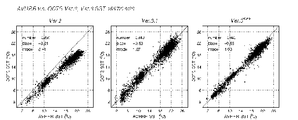
The comparison of the AVHRR data and the SST data estimated from the measurement data is shown in Fig. 5.

Fig. 5 Error distribution between OCTS SST and measured SST (after H. Murakami)

4 Conclusions

We presented a calibration and validation results of the version 3 products. We have also presented the coefficients used in the version 3 products. We confirmed that the version 3 products are accurate enough for scientific use (Fig 6 for CHL-a and Fig. 7 for SST map near Japan of April 26 1997). The representative accuracies are as follows: CHL-a estimation accuracy, 68%; water-leaving-radiance estimation accuracy, 94%; SST accuracy, 0.70K; and geometric accuracy, 1.3 km.

References

[1] NASDA document, "OCTS description and database," prepared by Mitsubishi electric cooperation, March 1994.

[2] T. Nakajima,

[3] Kishino, "

[4] H. Fukushima,

[5] H. Oaku, et. al., "Calibration and validation of OCTS," submitted to EUROPT'97

[6] Y. Mitomi, et. al., "".

[7] NASDA contract report by NEC, "Initial evaluation of OCTS," 1997 Sept.Appendix 1 Radiometric conversion for Ocean color

A.1.1 Process flow

The databases used for the radiometric calibration and validation are summarized. A flowchart to convert DN to the input radiance is shown in Fig. A-1.

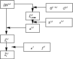
Fig. A-1 A flowchart for converting DN to input radiance (Visible and infrared band).

A.1.2 Calibration coefficients

bij gradient of the detector normalization slope -> Table III (gain_slope.data1)

cij offset of the detector normalization slope -> Table IV (gain_off.data1)

Lcij radiance at the two regions' boarder -> Table V (gain_cri.data)

Oij basic offset of the detector normalization -> Table I (Offsets)

Gij gain of the calibration coefficients -> Table II-1 (gain_base0-ocean normal)

-> Table II-2 (gain_base0-ocean high)

-> Table II-3 (gain_base0-land normal)

-> Table II-4 (gain_base0-land high)

A.1.3 Validation coefficients (algorithm tuning)

fj Amplification factor -> Table VI

ej Offsets -> Table VII

Appendix 2 Radiometric conversion for Sea Surface Temperature

A.2.1 Process flow

The data base used for the radiometric calibration and validation is summarized. A flowchart to convert DN to the input radiance is shown in Fig. A-2.

Fig. A-2 Flowchart to convert DN to the input radiance (Visible and infrared bands).

A.2.2 Calibration coefficients

aij detector normalization factor -> Table VIII

f() conversion table -> Table IX

A.2.3 Validation coefficients

gj empirical conversion coefficients -> Table X

Table I Offsets

0.795 0.639 0.036 0.090 0.000 0.486 0.000 3.570

0.450 0.036 0.467 0.915 0.000 1.421 0.831 2.893

0.839 0.775 0.065 1.197 0.478 0.000 1.314 0.396

0.228 0.529 1.142 1.255 0.088 0.650 0.246 7.667

0.510 0.341 0.860 0.133 0.025 0.000 0.494 0.000

0.333 0.017 1.163 0.856 0.050 2.761 2.151 0.000

0.478 0.071 1.036 2.418 0.669 2.575 1.097 0.000

0.499 0.089 0.096 0.000 0.916 1.021 1.099 5.335

0.863 0.187 1.431 0.595 0.000 1.428 2.098 2.272

1.013 0.017 1.571 1.577 0.186 2.338 1.990 0.346

/*

Table II-1 gain_base0 (Ocean-normal)(W/m2/str/mm)

6.01 6.09 7.29 8.19 10.45 16.10 23.81 48.84

6.01 6.09 7.29 8.19 10.45 16.10 23.81 48.84

6.01 6.09 7.29 8.19 10.45 16.10 23.81 48.84

6.01 6.09 7.29 8.19 10.45 16.10 23.81 48.84

6.01 6.09 7.29 8.19 10.45 16.10 23.81 48.84

6.01 6.09 7.29 8.19 10.45 16.10 23.81 48.84

6.01 6.09 7.29 8.19 10.45 16.10 23.81 48.84

6.01 6.09 7.29 8.19 10.45 16.10 23.81 48.84

6.01 6.09 7.29 8.19 10.45 16.10 23.81 48.84

6.01 6.09 7.29 8.19 10.45 16.10 23.81 48.84

*/

/*

Table II-2 gain_base0 (ocean-high)(W/m2/str/mm)

9.01 9.14 10.97 12.29 15.59 23.55 34.78 71.52

9.01 9.14 10.97 12.29 15.59 23.55 34.78 71.52

9.01 9.14 10.97 12.29 15.59 23.55 34.78 71.52

9.01 9.14 10.97 12.29 15.59 23.55 34.78 71.52

9.01 9.14 10.97 12.29 15.59 23.55 34.78 71.52

9.01 9.14 10.97 12.29 15.59 23.55 34.78 71.52

9.01 9.14 10.97 12.29 15.59 23.55 34.78 71.52

9.01 9.14 10.97 12.29 15.59 23.55 34.78 71.52

9.01 9.14 10.97 12.29 15.59 23.55 34.78 71.52

9.01 9.14 10.97 12.29 15.59 23.55 34.78 71.52

*/

/*

Table II-3 gain_base0 (land-normal)(W/m2/str/mm)

6.02 6.09 3.82 3.39 3.05 3.63 4.15 4.93

6.02 6.09 3.82 3.39 3.05 3.63 4.15 4.93

6.02 6.09 3.82 3.39 3.05 3.63 4.15 4.93

6.02 6.09 3.82 3.39 3.05 3.63 4.15 4.93

6.02 6.09 3.82 3.39 3.05 3.63 4.15 4.93

6.02 6.09 3.82 3.39 3.05 3.63 4.15 4.93

6.02 6.09 3.82 3.39 3.05 3.63 4.15 4.93

6.02 6.09 3.82 3.39 3.05 3.63 4.15 4.93

6.02 6.09 3.82 3.39 3.05 3.63 4.15 4.93

6.02 6.09 3.82 3.39 3.05 3.63 4.15 4.93

*/

/*

Table II-4 gain_base0 (land high)(W/m2/str/mm)

9.02 8.43 5.76 5.11 4.58 5.41 6.21 7.35

9.02 8.43 5.76 5.11 4.58 5.41 6.21 7.35

9.02 8.43 5.76 5.11 4.58 5.41 6.21 7.35

9.02 8.43 5.76 5.11 4.58 5.41 6.21 7.35

9.02 8.43 5.76 5.11 4.58 5.41 6.21 7.35

9.02 8.43 5.76 5.11 4.58 5.41 6.21 7.35

9.02 8.43 5.76 5.11 4.58 5.41 6.21 7.35

9.02 8.43 5.76 5.11 4.58 5.41 6.21 7.35

9.02 8.43 5.76 5.11 4.58 5.41 6.21 7.35

9.02 8.43 5.76 5.11 4.58 5.41 6.21 7.35

*/

Table III gain_slope.data1

1.924e-03 1.878e-03 2.430e-03 2.268e-03 8.700e-03 2.173e-02 2.899e-02 3.328e-02

5.491e-04 2.886e-04 1.420e-03 1.349e-03 6.950e-03 1.458e-02 1.187e-02 6.900e-02

3.290e-04 1.938e-04 7.084e-04 1.081e-03 2.409e-03 -4.414e-03 2.035e-03 2.825e-02

-8.055e-05 -1.067e-04 4.205e-04 6.220e-04 1.141e-03 8.971e-03 -1.887e-04 2.670e-02

-0.000e+00 -2.843e-17 -7.723e-17 4.480e-17 -4.642e-16 7.957e-16 -5.036e-18 -7.733e-16

-1.751e-04 -3.546e-04 -1.584e-04 2.630e-05 -1.400e-02 6.836e-03 -1.790e-02 -1.316e-02

-1.233e-04 -2.532e-04 -2.449e-04 1.398e-04 1.443e-04 9.463e-03 -7.544e-03 -4.519e-02

-5.318e-05 -1.300e-04 -1.823e-04 -3.984e-04 7.819e-05 6.749e-03 -5.816e-05 5.561e-02

2.042e-05 2.906e-04 3.237e-04 -7.054e-05 -6.178e-03 7.888e-03 -1.286e-02 2.095e-02

2.954e-04 7.677e-04 9.302e-04 6.460e-04 1.334e-03 1.220e-02 -7.916e-03 3.206e-02

Table IV gain_off.data1

1.0396 1.0404 0.99825 1.0001 0.98247 0.95390 0.98257 0.96288

1.0130 1.0214 0.99911 0.99950 0.98570 0.97425 0.99784 0.96450

0.99925 1.0068 1.0023 0.99372 0.99086 1.0109 1.0039 0.97428

0.99938 0.99656 1.0015 0.99600 0.99179 0.97272 1.0065 0.97200

1.0000 1.0000 1.0000 1.0000 1.0000 1.0000 1.0000 1.0000

1.0061 1.0036 1.0014 0.99883 1.0348 0.97966 1.0294 1.0141

1.0095 1.0047 1.0044 1.0013 0.99576 0.97255 1.0087 1.0477

1.0141 1.0192 1.0021 1.0029 1.0007 0.98191 1.0043 0.96488

1.0230 1.0259 1.0072 1.0053 1.0313 0.97790 1.0219 0.97535

1.0371 1.0507 1.0109 0.99999 1.0039 0.97420 1.0223 0.96054

Table V gain_cri.data

1000.0 1000.0 1000.0 1000.0 4.3132 2.3050 1.1184 0.96497

1000.0 1000.0 1000.0 1000.0 3.4964 2.3147 1.0242 0.58696

1000.0 1000.0 1000.0 1000.0 4.6238 2.0176 1.0421 0.91042

1000.0 1000.0 1000.0 1000.0 4.5604 2.8178 1000.0 1.1985

1000.0 1000.0 1000.0 1000.0 0.0000 0.0000 1000.0 0.0000

1000.0 1000.0 1000.0 1000.0 2.4500 3.2675 1.3655 0.61841

1000.0 1000.0 1000.0 1000.0 22.447 2.9004 1.1498 1.0548

1000.0 1000.0 1000.0 1000.0 54.910 3.4208 1000.0 0.63148

1000.0 1000.0 1000.0 1000.0 3.4452 3.8160 0.77273 1.1763

1000.0 1000.0 1000.0 1000.0 1000.0 2.9319 0.044229 0.98093

Table VI Amplification factor

1.1095279 1.0080781 0.9443458 1.0075835 1.0369337 0.9277923 0.9048486 0.764515

Table VII Offsets

0 0 0 0 0 0 0 0

Table VIII normalization factor (SST)

1.0004374 0.99741285 0.99692435 0.99922403

0.99380308 0.99855709 0.99830716 0.99931177

0.99506745 0.9989685 0.99962235 0.99948338

0.99424178 1.00066825 1.0002982 1.00142693

1 1 1 1

1.0003703 1.00006226 0.99990042 0.99979971

0.99560993 0.99917597 0.99897734 0.99997979

0.99707445 0.99809563 0.99817961 1.0013679

0.99344553 0.99737136 0.9977094 1.00178284

0.98483269 0.99610934 0.99531633 1.00143665

Table IX :

Temperature(K) #9 #10 #11 #12

2.200000e+02 1.185682e-03 6.010673e-01 1.247574e+00 2.169465e+00

2.201000e+02 1.194967e-03 6.031693e-01 1.250950e+00 2.174886e+00

2.202000e+02 1.204317e-03 6.052767e-01 1.254333e+00 2.180316e+00

2.203000e+02 1.213732e-03 6.073896e-01 1.257721e+00 2.185754e+00

2.204000e+02 1.223213e-03 6.095079e-01 1.261115e+00 2.191201e+00

2.205000e+02 1.232759e-03 6.116317e-01 1.264516e+00 2.196657e+00

2.206000e+02 1.242371e-03 6.137609e-01 1.267923e+00 2.202122e+00

2.207000e+02 1.252050e-03 6.158956e-01 1.271335e+00 2.207595e+00

2.208000e+02 1.261796e-03 6.180359e-01 1.274754e+00 2.213077e+00

2.209000e+02 1.271609e-03 6.201816e-01 1.278179e+00 2.218568e+00

more data are provided in the file (NEW.TIR)

Table X :

i 1 2 3 4 5 6

g -29.553529 1.1118699 4.2586536 -0.6445829 1.4122749 -0.5512104

Table XI

band9 band10 band11 band12

0.8 0.0 1.9 1.0

0.9 0.4 1.4 0.9

1.5 1.0 2.4 0.2

0.6 2.7 1.5 0.0

1.4 2.5 1.6 0.7

1.3 0.1 2.0 1.5

1.7 1.3 1.0 0.9

0.5 1.0 1.0 0.3

0.1 3.2 0.6 1.2

0.0 3.6 1.0 0.3

Appendix. Radiometric Conversion from Previous Version to This Version

TBD

Appendix 3 Exact expression of Fdata

Exact expression of Fdata is given by

(A-1)

where h is the reflection coefficient of the scanning mirror, bd, bp, bam, bad are the factors correcting the temperature dependency, k is the number for tilt. However, bs (bd, bp, bam, bad) are negligibly small and set to be zero.

Table A.1 Reflection coefficients (h)

tilt angle

band -20(k=0) 0(k=1) 20(k=2)

1 0.974 1.000 0.980

2 0.984 1.000 0.997

3 0.990 1.000 0.997

4 0.992 1.000 0.996

5 0.994 1.000 0.995

6 0.995 1.000 0.995

7 0.996 1.000 0.995

8 0.996 1.000 0.995

9 1.000 1.000 1.003

10 1.008 1.000 0.992

11 0.982 1.000 0.992

12 0.975 1.000 0.981