About TANSO-FTS
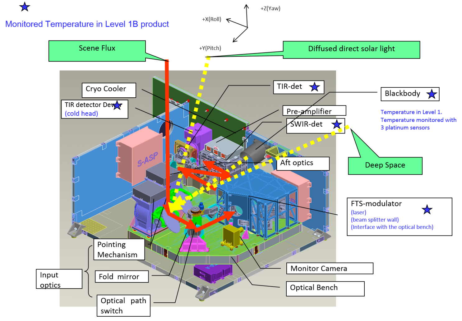
There are three units in TANSO-FTS; an optics unit, a control unit, and an electronics unit. The optics unit consists of a pointing mechanism, a monitor camera (CAM), relay optics, a TANSO-FTS mechanism, detectors, and analog-signal processors. All the optical components are mounted on the optical bench, of which temperature is controlled at 23 degrees C and kept between 20 and 26 degrees C. On the optics unit structure, a cooler for a TIR detector, a blackbody, a diode laser for ILS calibration, a diffuser plate and its driving mechanism, a hood to minimize the stray lights, and analog electronics are mounted. The control unit consists of a TANSO-FTS controller, a pointing mechanism controller, a detector temperature controller, and cooler controller electronics. The electronics unit has functions for heater-controlling, data processing, and a data-telemetries-commands-transmission interface with the satellite bus system. All the components of the electronics unit have redundancy.
Main Specifications of TANSO-FTS| FOV | IFOV 15.8 mrad (10.5 km on the ground at nadir) Coverage (cross track ±35 degrees, along track ±20 degrees) |
|||
|---|---|---|---|---|
| Aperture | 68 mm | |||
| Speed | 1.1, 2, 4 sec/interferogram | |||
| MOPD | ±2.5 cm (both sides) (maximum optical path difference) | |||
| band | 1P, 1S | 2P, 2S | 3P, 3S | 4 |
| Coverage (cm-1) | 12900-13200 | 5800-6400 | 4800-5200 | 700-1800 |
| Spectral resolution FWHM (cm-1) (Measured P(S)) | 0.367(0.356) | 0.258(0.257) | 0.262(0.263) | 0.24 |
| Detector | Si | InGaAs | InGaAs | PC-MCT |
| SNR (prelaunch) (Measured) | >340 | >320 | >410 | >280 |
| Onboard Calibration | Solar irradiance, Deep Space, Lunar (radiance), Diode laser (ILS) | Black body, deep space (Radiance) | ||
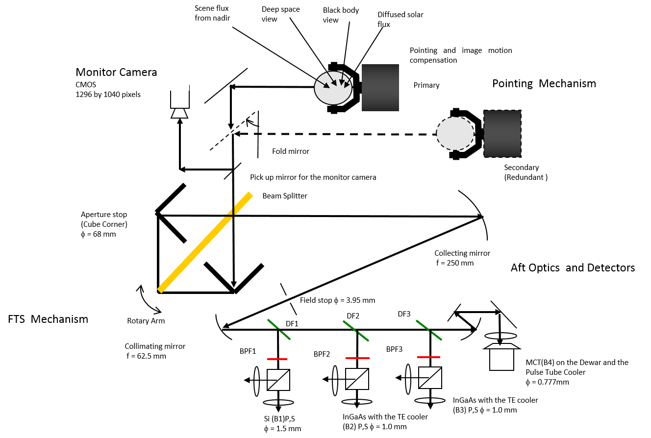
Schematic layout of the TANSO-FTS optical system. Since January 2015, the scene flux has been introduced from the secondary pointing mechanism.
TANSO-FTS Observation Principle
In order to monitor Green House Gases (GHGs), it is essential to measure the troposphere where greenhouse effect occurs. In general, it is more difficult to measure the troposphere from space than the stratosphere, because scattering by cloud-and-aerosol and the height of the earth surface have to be considered. Limb viewing methods such as limb emissions and solar occultation is not capable of lower troposphere measurements. A down-looking measurement is the only feasible way to measure GHGs by detecting the flux that passes through the lower troposphere. Therefore GOSAT accommodates the down-looking instruments, TANSO-FTS and CAI, to measure GHGs and detect cloud and aerosol.
TANSO-FTS measures the scene radiance of solar short wave infrared spectra (SWIR) reflected on the earth’s surface. Column density of CO2 is mainly retrieved from the 1.6 µm region absorption lines, of which intensities are less temperature dependent. The 2.0 µm region can also be used for CO2 retrieval. In addition, CH4 is retrieved in the 1.6 µm region. The Oxygen (O2) A band absorption at 0.76 µm are used to estimate the effective optical path-length, which is a key parameter for the column density retrieval. As O2 concentration is constant, well known, and uniformly distributed throughout the atmosphere, it can be used as a reference. We have added measurement of thermal infrared spectra (TIR) radiated from the ground and the atmosphere to retrieve the vertical profile by acquiring the absorption lines of various cross-sections.
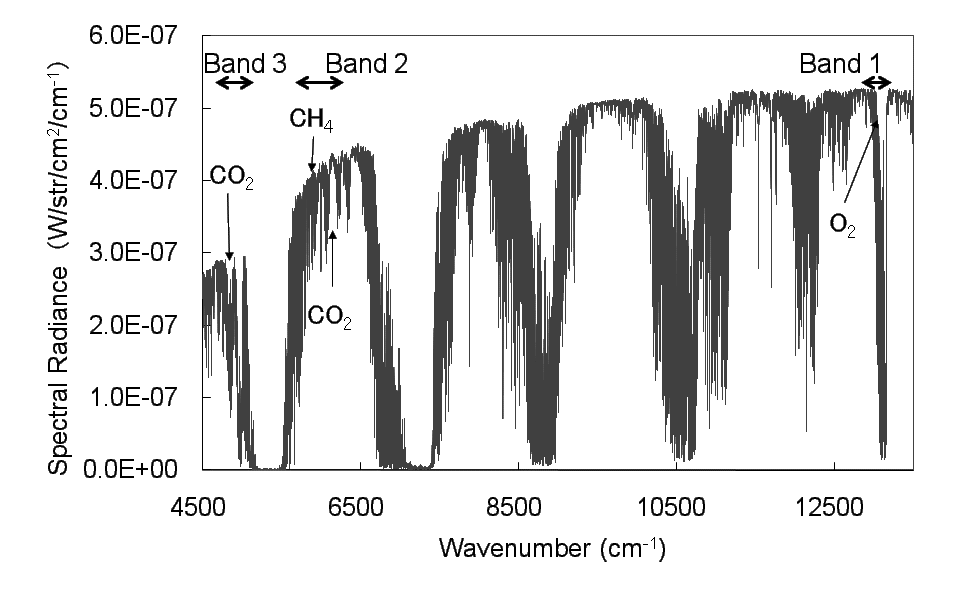
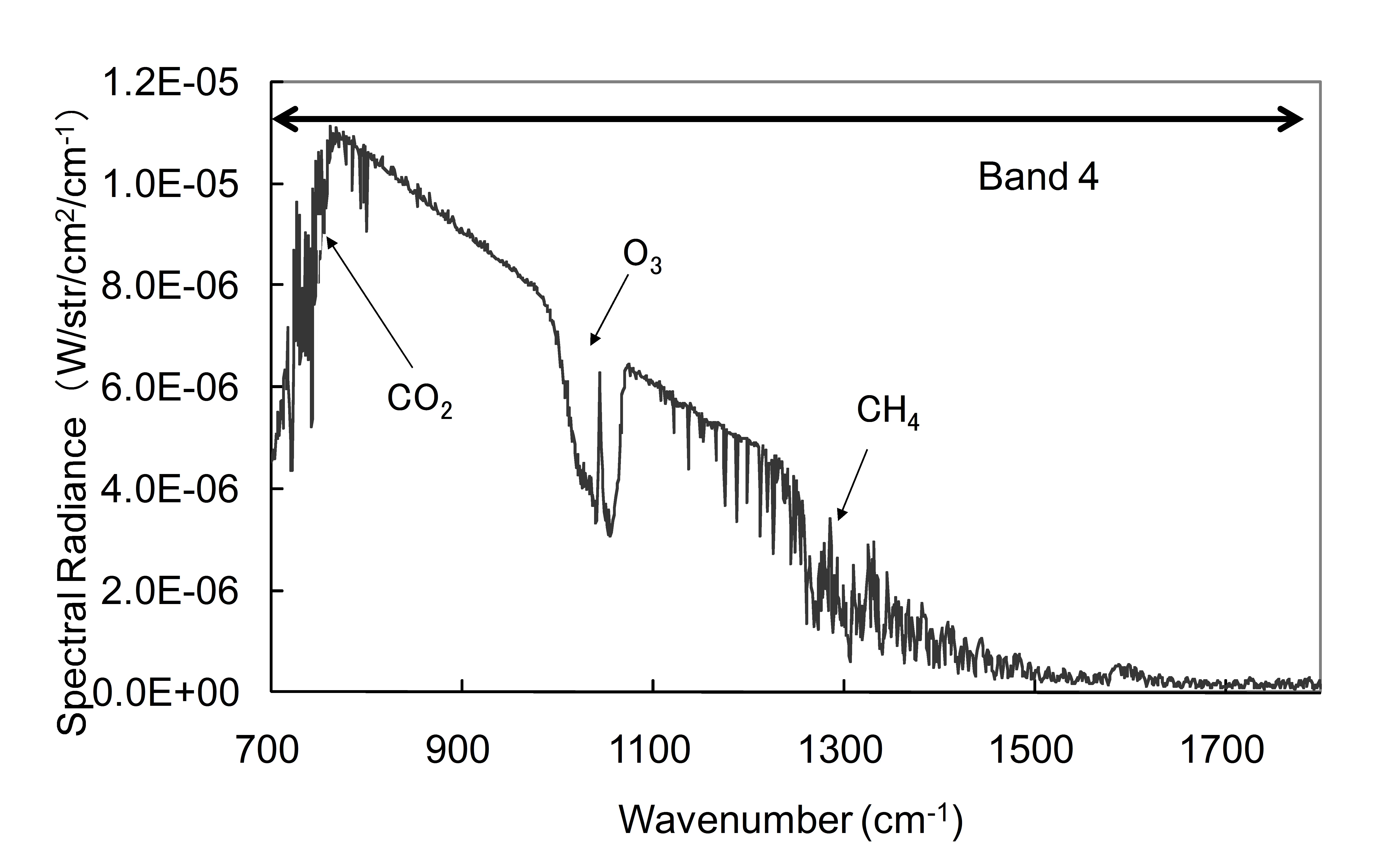
Simulated spectral coverage of TANSO-FTS; (a) SWIR (Bands 1, 2, and 3) and (b) TIR (Band 4).
Fourier Transform Spectrometer Mechanism
The FTS-mechanism is a double pendulum type interferometer with two cube-corner reflectors, which create a ±2.5 cm optical-path-difference (OPD) four times as long as the mechanical motion. The two cube-corner reflectors are mounted at the edges of a rotary arm. They are carefully aligned with each other to maximize modulation efficiency with the minimum optical shear permanently. The arm is mounted on the beam splitter holder with a flexible blade and actuated with a rotary motor. The two cube-corner reflectors and the motor are statically balanced in all three axes and robust against vibrations. The rotary arm mechanism moves smoothly with better than 1% speed stability, creating uniform frequency of the output modulated-signal. In order to obtain high SNR, the sampling electrical bandwidth has to be small enough, in other words, the scan speed has to be slow enough. At least 4 sec is needed to achieve the required SNR and the nominal time for one way interferogram acquisition is set at 4 sec. TANSO-FTS has a fully redundant sampling system with two 1.31 µm distributed-feedback (DFB) lasers and two InGaAs detectors. Each diode laser has a much longer life span than a conventionally used HeNe laser and its size is small enough to have redundancy. As the diode laser wavelength has temperature dependency, its temperature is well controlled with stability of 25.000±0.001 degrees C with a thermo electric controller. So the wavelength stability (Δλ/λ) is better than 10-7, which is equivalent to typical HeNe laser stability.
Aft-optics and Detector
Modulated light from the FTS-mechanism is collected into a circular stop. Geometric registrations between seven spectral bands of TANSO-FTS are well aligned by sharing this common field stop. It defines IFOV of 15.8 mrad, which is equal to the 10.5 km footprint for nadir pointing. To maximize the optical throughput, IFOV corresponds to maximum divergence allowed at the most important band 2 for 0.2 cm-1 spectral resolution (interval). The scene flux is collimated and divided into four spectral bands with dichroic filters. The three dichroic filters reflect the shortest wavelength band light and transmit the longer wavelength bands light. These filters are carefully designed to minimize the polarization sensitivity of SWIR bands and minimize background radiation of TIR. Each SWIR-band light passes through a narrow band-pass filter and is divided into two detectors by a polarization beam splitter. The narrow band-pass filters are wedged to avoid channeling and reject shorter wavelength light to avoid aliasing and minimize out-of-the-band stray light.
Two Si detectors are applied for bands 1P and 1S. The four InGaAs detectors for bands 2 P, S and 3 P, S are non-biased and cooled at -40 °C with three-stage thermoelectric coolers to minimize dark currents. The TIR light is collected on a single Photo-Conductive (PC) HgCdTe (MCT) detector, which is mounted on the dewar and cooled at 70 K with a pulse tube cooler. The pulse tube cooler has a very low vibration level with no impact on the interferogram acquisition and it also has a variable motor frequency to minimize unexpected vibration interference on orbit.
Signal Processing and Data Transmission
Each detector signal current is converted to voltage and amplified with operational amplifiers. To minimize high frequency noise, multi-stage amplifiers with low pass filters are integrated. Then analogue signals are converted in parallel to digital data with one 16bit-AD converter per detector. Therefore, seven interferograms are acquired simultaneously. For bands 1, 2, and 3, up-and-down zero-crossings of the laser-fringes are utilized for sampling triggers, which results in 76,336 sampling points per interferogram with the half laser wavelength (λ/2) interval. Band 4 samples 38,168 points per interferogram with λ interval. For band 1, to avoid aliasing of noise, only a modulated portion (AC) is acquired. For bands 2 and 3, AC plus offset data (DC) are acquired. For band 4, both the modulated portion (AC) and non-modulated portion (DC) are acquired and amplified separately. The DC portion is used to correct the non-linearity effect of the PC-MCT detector. Digital signals are processed in the electronics unit. In addition, telemetry data used for level 1 and 2 processing is added to the data header. The telemetry data include the satellite position, GPS time, amplifier gain levels, AT and CT angles of the pointing mechanism, and the temperature of the blackbody and the detectors. Finally, acquired data are transmitted to the MDP of the GOSAT satellite bus system in Consultative Committee for Space Data Systems (CCSDS) format.
Pointing System
TANSO-FTS’s two-axis pointing mechanism has a pointing function for the cross track (CT) and along track (AT) directions, allowing precise viewing of the earth and the calibration sources. By mainly rotating the CT stepper motor, the pointing mechanism views the Earth’s surface, deep space, the blackbody, and the diffuser. To point at any target on the Earth’s surface within a 3 day revisit cycle, a scan angle covers ±35 degrees from the nadir. By mainly rotating the AT motor, TANSO-FTS can view the same field to compensate the satellite motion during one way interferogram acquisition time between turnarounds, which is typically 4 sec (image motion compensation, IMC). The motion of the pointing mechanism is synchronized with the FTS mechanism. Both the AT and CT motors are actuated and settled down within rotary arm turnaround of the FTS mechanism, which is between 0.4 and 0.6 sec. In nominal observation mode, the pointing mirror views predefined grid points of the earth close to nadir. Over the ocean where surface reflectance is small, the pointing mechanism views widely spread sun-glint area where specular reflection occurs and reflectance is high (sun-glint observation mode). As the AT viewing angle range is ±20 degrees, sun-glint observation is limited to low and middle latitudes. The primary pointing system was switched over to the secondary backup system on 26 January 2015. Hence the TANSO-FTS Level 1 data taken after January 2015 are of the secondary pointing system.
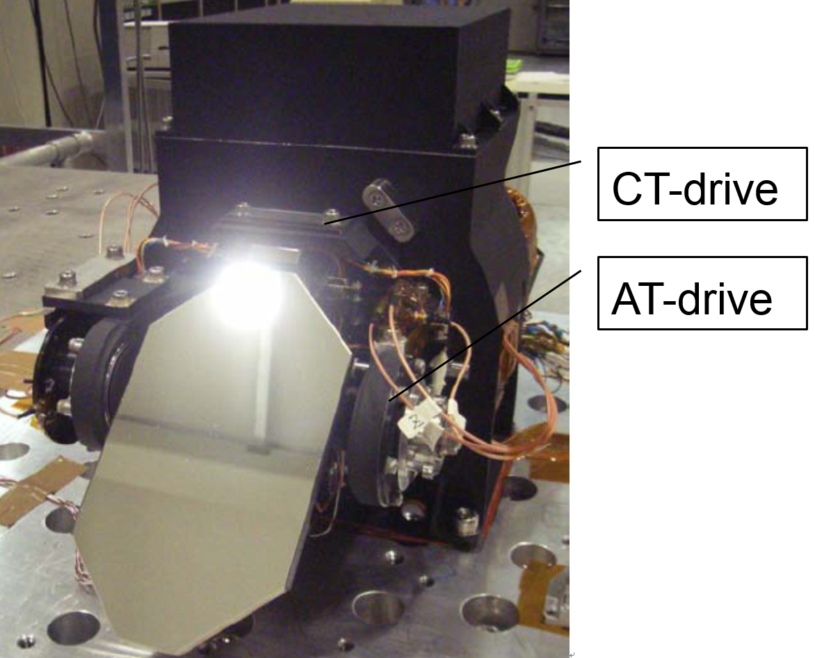
Photo of the TANSO-FTS 's two-axis pointing mechanism
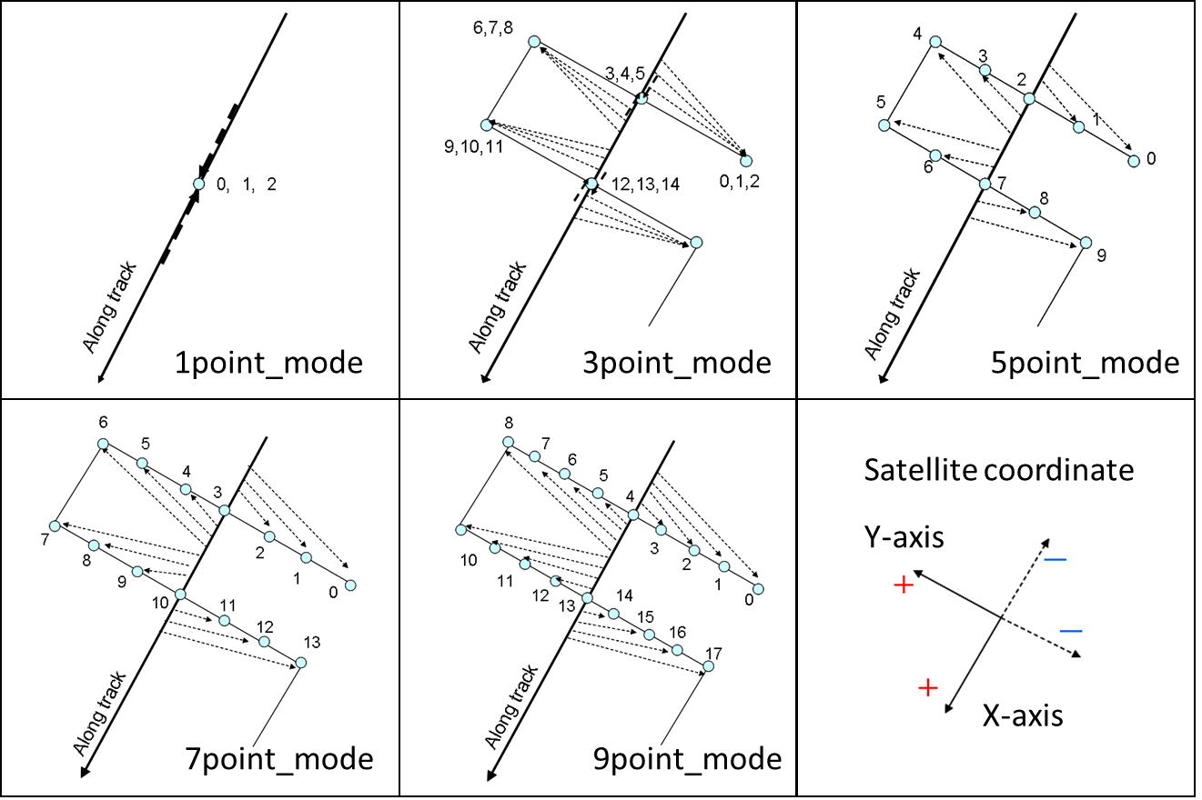
Grid observation patterns
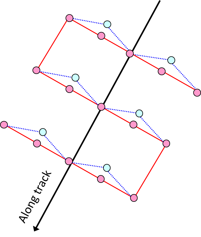
an M shape grid overwritten on the 5-point
cross-track scan mode used between Jun. 26, 2009 and Jul.31, 2010
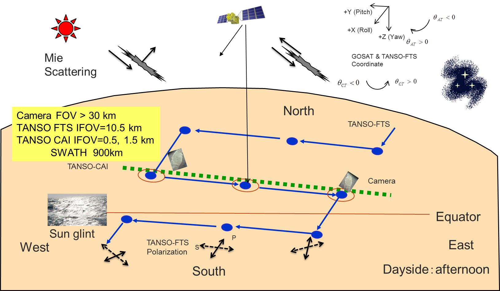
Observation geometry of TANSO-FTS and the monitor camera (the 3-point cross-track scan mode), and TANSO-CAI.

Monitor Camera (CAM)
A small 2 dimensional CMOS camera is installed to register the TANSO-FTS instantaneous field of view (IFOV). Careful alignment and rigid mounting of the monitor camera on the optical bench before launch stabilizes registration between the centers of TANSO-FTS IFOV and the monitor camera before and after the launch, which will be kept over the GOSAT mission. By comparing on-orbit TANSO-CAI and monitor camera images, the registration between CAI and TANSO-FTS can be estimated. The registration has to be estimated with an accuracy of 250 m. This estimated registration can be validated by viewing Ground Control Point (GCP). The monitor camera has a wider field of view and higher spatial resolution than the TANSO-FTS single pixel. The size of the image and acquisition interval can be selected by the command from the ground. By setting the same sampling interval as the interferogram acquisition such as 4 sec, a scene image of each interferogram can be acquired. The camera data are transmitted to the Mission Data Processor (MDP).
Main Specifications of the Monitor Camera on TANSO-FTS| Optics (focal length) | 45.5 mm |
|---|---|
| Aperture | 5 mm |
| Detector | 2 dimensional CMOS (about 1,300,000 pixels) |
| VGA mode | 640 by 480 frame rate > 5fps (frame per sec) |
| SXGA mode | 1280 by 1024 frame rate > 5fps |
| IFOV | < 100 m |
| FOV | > 2.58 deg |
Target Observation
Occasionally by uploading the observation start time and the set of pointing angles from the ground, TANSO-FTS can view targets between AT angle of ±20 degrees and CT angle of ±35 degrees for validation, vicarious calibration, large emission sources such as mega cities, active volcanos, oil and gas fields, livestock, and landfills. Pointing patterns are registered on the onboard tables, which has up to 3,000 pairs of the CT and AT angles.
The research teams engaged in Research Announcement and JAXA operators may submit requests for target observations. Since there is a limit in the number of target observation points that can be stored in the onboard memory and a new target may interrupt the continuous observations of other important targets, not all requests from RA users are adopted. The deadline of the target observation requests (from NIES which collects and coordinates individual RA user requests) for week N is 10:00 JST (1:00 UTC) on Wednesday in week N-6. Small changes can be made after the basic observation plan for week N has been determined at the end of week N-5. The observation plan for day D, however, can no longer be altered after day D-3 because of the lack of time for preparing and uploading commands to TANSO.

Observation geometry of TANSO-FTS in the Target mode
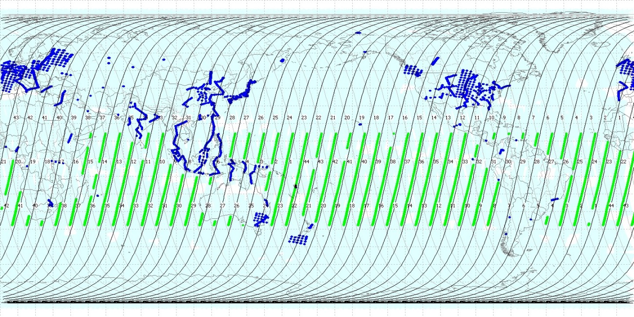
An example of the TANSO-FTS observation pattern. The green points show sun-glint observation points and the blue points show target observation points.
Temperature Control
The temperature of both TANSO-FTS and CAI optics is controlled at 23±3 degrees C. As the modulation efficiency of the FTS-mechanism is temperature-dependent, stability within a 98 min orbit period, which is the solar irradiance calibration interval, is important for consistent response within an orbit period. The temperature variation within 98 min is about 0.1 K and the response instability is negligibly small.
Level 1 Processing Algorithm
All the unprocessed numerical form interferograms are saved as Level 1A data. The payload correction data from the satellite bus and telemetry data of TANSO-FTS are added in both Levels 1A and 1B products together with the measured data. These data include the time stamp, the satellite and sun position, the geolocation, the AT and CT angles of the pointing mirror, the detector temperature, the blackbody temperature, and gain level, all of which are necessary for data processing and analysis. The time stamp in the data shows the start of the interferogram acquisition. The satellite position is interpolated by using the payload correction data, which is transmitted from the satellite every second. The AT, CT, solar angles, and the geometry information are acquired at the start of interferogram acquisition as well.
Interferogram of each band (two linear polarizations of Bands 1, 2, and 3 and scalar Band 4) is processed independently. TANSO-FTS Bands 1, 2, 3 (SWIR), and 4 (TIR) are processed as illustrated in below flowchart.
Click on the box in the flowchart to see an explanation of the corresponding data processing.
Description of the updates in the later released product versions is also available online at GDAS.
IGM Saturation Detection
For all 7 bands, interferograms with digital number (DN) values that exceed 65,400 are screened and their ZPD saturation flags are set. The threshold was set to a slightly lower value than the actual dynamic range in order to provide some margin. For Band 4, there is also a lower saturation threshold of 136.
IGM DN-to-V Conversion
DN values of each interferogram are converted to physical quantity (Volts), namely analog values. For Band 4, both AC and DC components of an interferogram are recorded and each of them is converted separately.
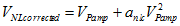
Nonlinearlity Correction (TIR)
There are three blocks in the signal electronics: namely the detector, analog circuit, and ADC. Among these, the detector is the largest source of nonlinearity. The Si detectors of Band 1 and the InGaAs detectors of Bands 2 and 3 are adequately linear but the PC-MCT detector of Band 4 has nonlinearity. The nonlinearity is corrected using a 2nd order polynomial. Assuming that nonlinearity characteristics do not change with time after launch, the coefficients can be determined from the well-characterized large photon input data under stable conditions in a vacuum chamber prior to launch. The nonlinearity corrected data  is calculated by equations (1) and (2) described below with the measured raw AC components of the interferogram in voltage VAC and DC voltage VDC. VDC is the average of DC samples, which are monitored at 38 samples per interferogram. We subtracted offset
  , which has a gradual increase since launch probably due to temperature change of the electric circuit. is estimated from the DS view data and modeled as a function of time since launch.
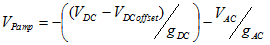 (1)
(1)
The gain factors  and
and  are 0.681 and 110.103, respectively.
 (2)
(2)
 is the nonlinearity correction coefficient of 0.6056.
Coase ZPD Detection
The ZPD position is determined by searching the center burst (peak) of the interferogram. It corresponds to the position of maximum value in the (DC-subtracted) interferogram for Bands 1, 2, and 3. For Band 4, the maximum absolute value in the AC component is searched because the peak could have a negative value in the TIR band. Detection of the ZPD position is performed for each band, although the ZPD position is in principle common in all of the 7 bands.
Note that the order of applying this processing has been changed (moved up) in L1B V201.201 (V201) for the proper spike and pointing fluctuation detection under largely shifted ZPD positions.
Gain Change and Spike Noise Detection and Correction, IGM Pointing Fluctuation Detection (SWIR)
Interferograms that have a jump (due to a gain change), spikes (possibly caused by cosmic rays), and significant fluctuations are screened and a quality flag is attached to the Level 1B data. The signal of a jump or spike found is replaced with an estimated DC signal which is the average of the interferogram levels acquired before and after the spike. Low frequency fluctuations seen on some interferograms are generated by the pointing mirror mechanism’s unstable settling down over non-uniform targets. The fluctuation is corrected in the subsequent “intensity variation correction” processing.
IGM Spike Noise Detection and Correction (TIR)
Interferograms that have spikes or significant fluctuations are screened. They are screened and a quality flag is attached to the Level 1B data. The signal of a spike is replaced with an estimated DC signal which is the average of the interferogram levels acquired before and after the spike.
Intensity Variation Correction
The intensity variation mainly caused by optical vignetting and pointing fluctuation is corrected by dividing (normalizing) the DC-coupled interferogram by its low frequency components. The normalized interferogram is subsequently multiplied by the DC level averaged near ZPD in order to maintain its magnitude information. In the process of normalization, the linear slope of the DC component in L1B V201 is used instead of the boxcar DC component in previous versions. This correction is applied only to Band 2 and 3 at this time.
IGM Saturation Detection
Saturation is detected by checking the low-frequency components near ZPD of the DC-coupled interferogram. A negative deviation from zero indicates the existence of saturation at center burst. Saturation can also occur at negative center burst in the TIR band, therefore a positive deviation is also checked in Band 4.
IGM DC Subtraction
Up to L1B V161, the DC level is subtracted by the linear slope obtained by averaging the 100 edge fringes at both ends of the interferogram. This process sometimes creates artifact spectra from the remaining linear slope component. For L1B V201, DC is subtracted by using a single point at the edge instead of averaging the 100 fringe value.
Fine ZPD Detection and Zero Filling for ZPD Shifted Side
In case of observing multiple peaks near the center of an interferogram and thus having difficulty in detecting its true ZPD position with amplitude alone, fringe count error (FCE) is estimated for each interferogram to adjust the coarse ZPD position determined earlier. The FCE value is determined so that the corresponding imaginary spectrum has a minimal structure. Only final ZPD values are stored in the Level 1B product.
OPD Sampling Interval Non-uniformity Correction
The ideal interferogram would be acquired with an equal sampling interval of the laser fringes within the entire optical path difference (OPD) range. The actual on-orbit interval, however, decreases nonlinearly with OPD. The error caused by this non-uniformity is close to the noise level in the forward direction data but slightly larger in the backward scan data.
The OPD sampling interval non-uniformity correction (SINUC) was applied in L1B V150. However, a spectral ringing artifact was inadvertently introduced to the spectra in the L1B V150 processing, as 100 zeros were filled in at both ends of the interferogram. The L1B V161 processing switched off SINUC to correct this mistake.
V201 applies SINUC again by modifying the sampling interval non-uniformity model to have smooth ends at the maximum OPD. This correction improves the consistency between the forward and backward scanning without the ringing artifact structure seen in V150.

Sampling interval non-uniformity as a function of OPD of the forward and backward scans.
Intensity Dependent Phase Delay Correction (Band 1)
After the release of L1B V150 and V161, we measured the intensity-dependent phase delay in the high gain amplifier circuit using the EM model in the laboratory [Suto et al. 2014]. In addition, we estimated the phase delay of the in-orbit circuit by finding the parameters that minimize out-of-band spectra. These phases are corrected separately by resampling the interferogram in L1B V201, while in V150 and V161 these phases in the high gain amplifier and amplitude nonlinearity in the low pass filter are simultaneously corrected by using a single set of 3rd order polynomials.

Band 1 analogue circuit block diagram.
 (solid line) and S (B1S) (dotted line) high gain analogue circuit. Higher gain B1S has larger dependency.")
Intensity dependent phase of the Band 1 P (B1P) (solid line) and S (B1S) (dotted line) high gain analogue circuit. Higher gain B1S has larger dependency.
Analog Circuit Nonlinearity Correction (Band 1)
The high gain of Band 1 uses a Chebyshev filter (low-pass filter) with much sharper gain peak and cut-off than the other bands to avoid aliasing of noise. Unfortunately, its gain is sensitive to the capacitance in the circuit, which varies with input voltage, temperature, and time. The nonlinearity induced by the input-voltage change can be corrected using a 3rd order polynomial. These coefficients are determined so that the out-of-band artifact spectra are minimized. The Band 1 nonlinearity correction was applied in L1B V150 and V161. However, it was found that the nonlinearity correction could not remove input-level dependent offset and out-of-band artifacts completely because both the high gain amplifier and low-pass filter circuit have nonlinearity with different characteristics. In L1B V201, the nonlinearity correction by the same method (using a 3rd order polynomial) is improved by isolating the correction of the intensity-dependent phase in the high gain amplifier.
Speed Instability Correction (Band 1)
The phase delay mismatch between the metrology laser electronics and science channel degrades the robustness to scan speed instability and creates artifacts in the spectra. Only the medium gain of Band 1, which is used over high reflectance regions such as the Sahara, Arabian and Australian deserts and solar calibration, has a significant delay mismatch. The speed instability is caused by a combination of two sinusoidal micro-vibration sources, namely, 244 Hz from the satellite attitude control’s earth sensor and the 325.5 Hz resonant frequency of the FTS mechanism. Since the nominal scan speed is very constant, these two additional modulations to the interferogram have quite pure sinusoidal variations and can be corrected by retrieving their amplitudes and phases for each interferogram acquired with medium gain. When each interferogram is processed, these four parameters are estimated to minimize the out-of-band artifact spectra. The interferogram is then interpolated at the expected sampling positions.
Backward IGM Reversing
The order of interferogram data in each backward scan is reversed so that its sequence is consistent with time.
Zero Filling for Prime Factor FFT, Weighting Function Application for ZPD-biased-interferogram
The number of interferogram data used for inverse Fourier transform is 76,336. On the other hand, a prime number-based combinations of 76,545 (=37×5×7) for Bands 1, 2, and 3 have been selected as the size of FFT. For Band 4, the number of interferogram data used and the FFT size for inverse Fourier transform are 38168 and 38,400 (=29×3×52), respectively. A zero-filling at both ends of the interferogram data is carried out to fill the balance of the FFT input vector.
A large ZPD shift causes a change in spectral resolution since the interferogram is not long enough on one side. To provide precisely uniform resolution data for the entire mission, a ZPD bias correction is introduced to produce the full spectral resolution data from the biased ZPD interferogram in L1B V201. The biased interferogram is multiplied by the weighting function and Fourier transformed using the same length as a normal interferogram. The smooth weighting at the edges are used to minimize the artifacts. The regions where the weight is 2 or 0 varies with the ZPD bias. When the ZPD shift is less than 100 half laser fringes, no weighting function is applied. After June 2014, almost all the data are processed with a weighting function resulting in a slight reduction of the signal to noise ratio (SNR) as the number of total sampling points per interferogram is reduced by the bias value. The constant ILSF can be applied to all the L1B V201 products. The ILSF model for V201 is provided from NIES GDAS.

Biased ZPD correction with weighting function for version 201.
I-FFT and Phase Correction (SWIR)
Conversion from interferograms to spectra with a prime factor I-FFT is performed, and is followed by phase correction. The phase can be retrieved from the ratio of the imaginary to the real spectra. At highly absorbed lines, the phase is very noisy and if used at full resolution it will be over-corrected. By significantly reducing the spectral resolution of the phase determination, a closer representation of the smooth phase structure is obtained. The reduced resolution phase is obtained with Gaussian apodization.
I-FFT (TIR)
Interferograms are converted to spectra with a prime factor I-FFT. Phase correction is not performed on TIR band data. The effect of emissions from the beam splitter (ZnSe) is considered negligible except for the longwave region near 14µm.
ZPD Crossing Time Calculation
The time stamp of the telemetry data is the turnaround completion time TTAT, which corresponds to the start of interferogram acquisition. The interferogram near ZPD is the most informative, and ZPD passing time is calculated using the following relationship:
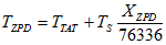 (3)
(3)
where TS is the scan duration and Xzpd is the ZPD position in the vicinity of the median of 1-76336.
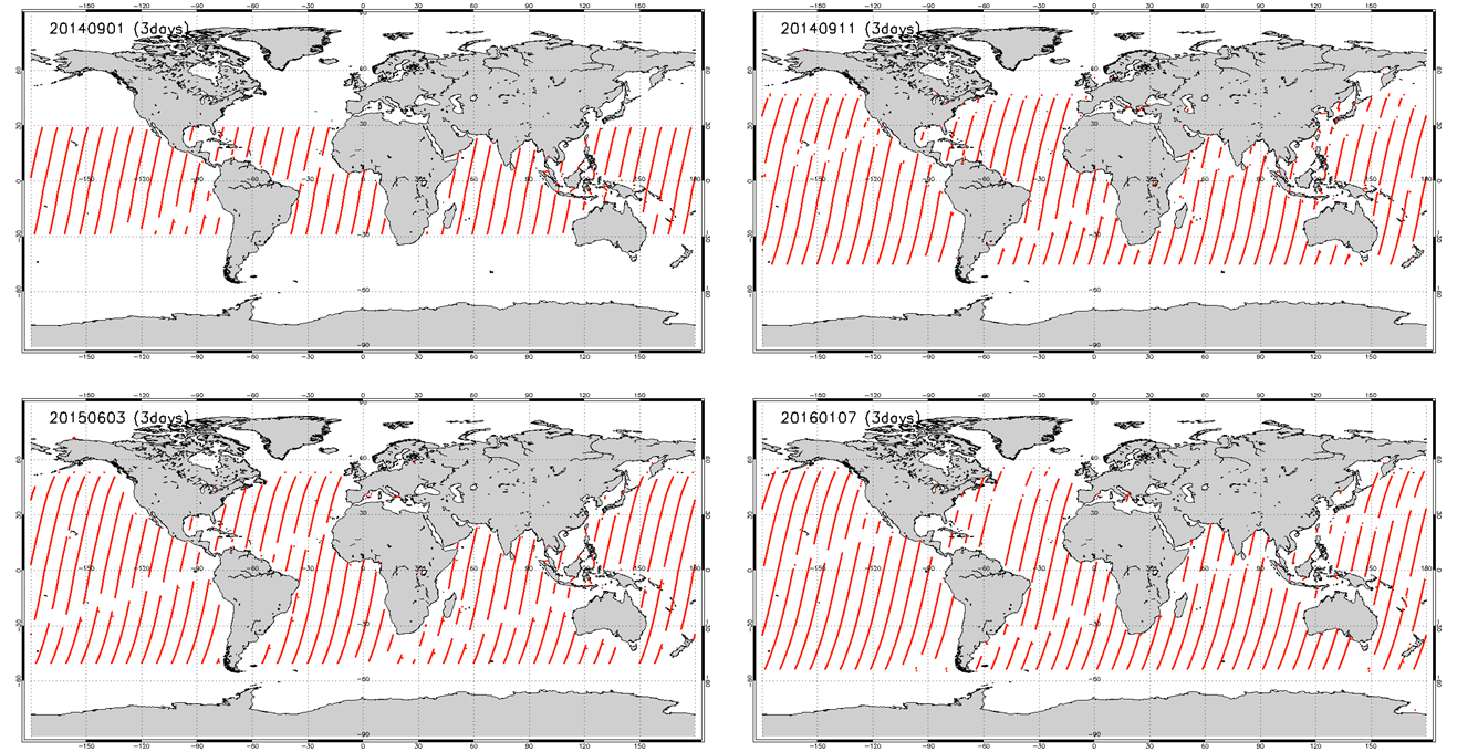
Radiometric and Polarimetric Calibrations (TIR)
Spectral radiances are calculated by the complex calibration with DS and BB spectra as expressed in Eq. (4).
 (4)
(4)
In the above equation,  ,
,  , and
, and  denote measured spectra of nadir observation, DS, and BB, respectively. The symbols
  and
and  are the wavenumber and scan direction of the FTS mechanism. The effective spectral radiance
  is calculated with the equation below.
 (5)
(5)
We use the emissivity  of 1 assuming that the environment temperature
  is close to the blackbody temperature. is further corrected for the polarization effect. The DS view obscuration correction introduced in L1B V130 has been removed since V161.
3-day recurrent period × 4-way operation patterns:
①(3-day) limited calibration and validation site(Until Jan. 11, 2016)
(3-day) sun glint and limited calibration and validation site(Since Jan. 12, 2016)
②(3-day) sun glint, calibration and validation site, RA target observations
③(3-day) sun glint and limited calibration and validation site
④(3-day) sun glint, calibration and validation site, RA target observations
Glint Observation Operation
Since Aug. 2, 2010
The image motion compensation is enabled during glint observation.
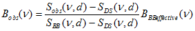
Before May 6, 2013
As the glint areas change with the direction of the earth's axis, glint observation points were planned at different seasons (every two months), by calculating the satellite positions from which the specular points can be observed.
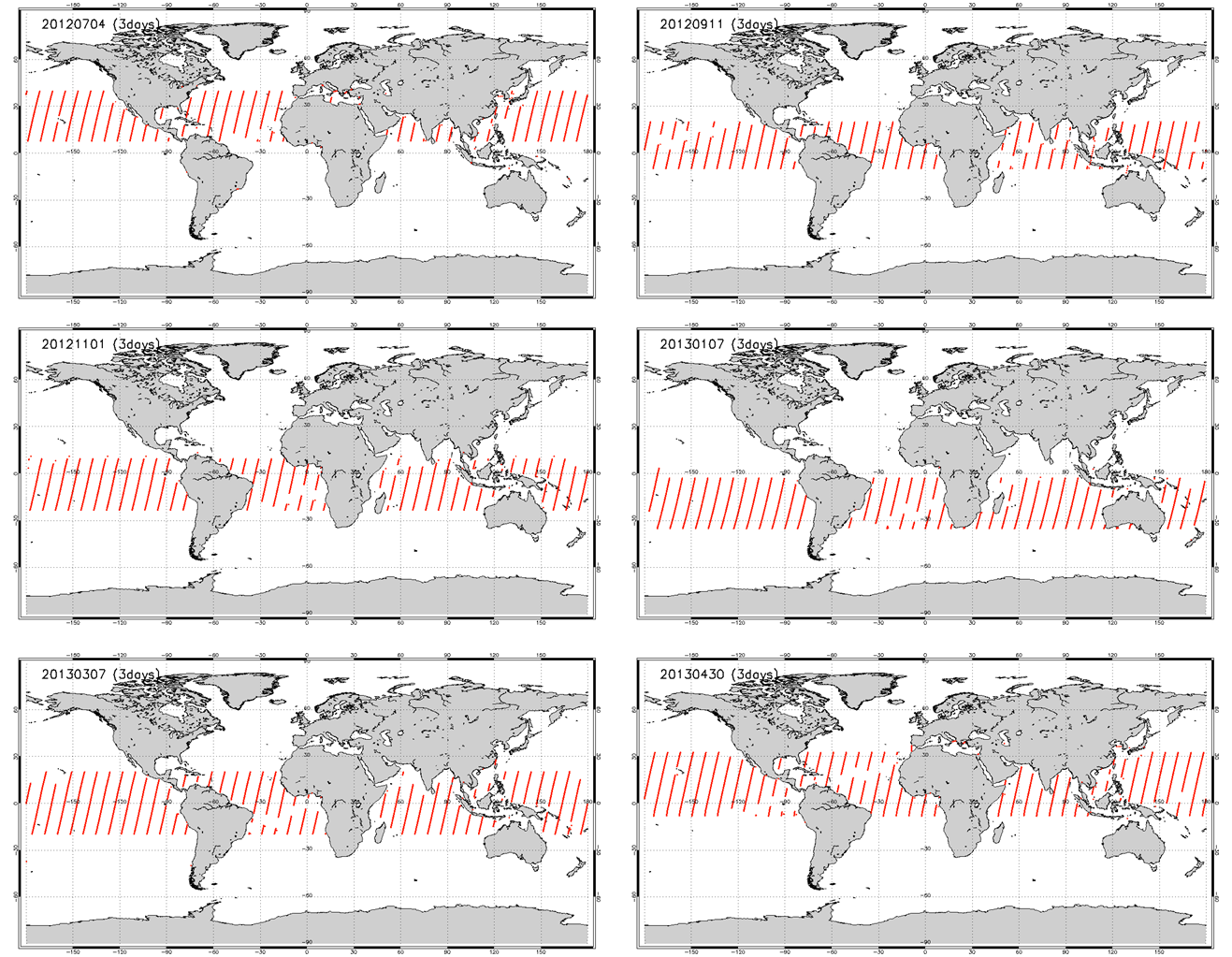
Since May 6, 2013
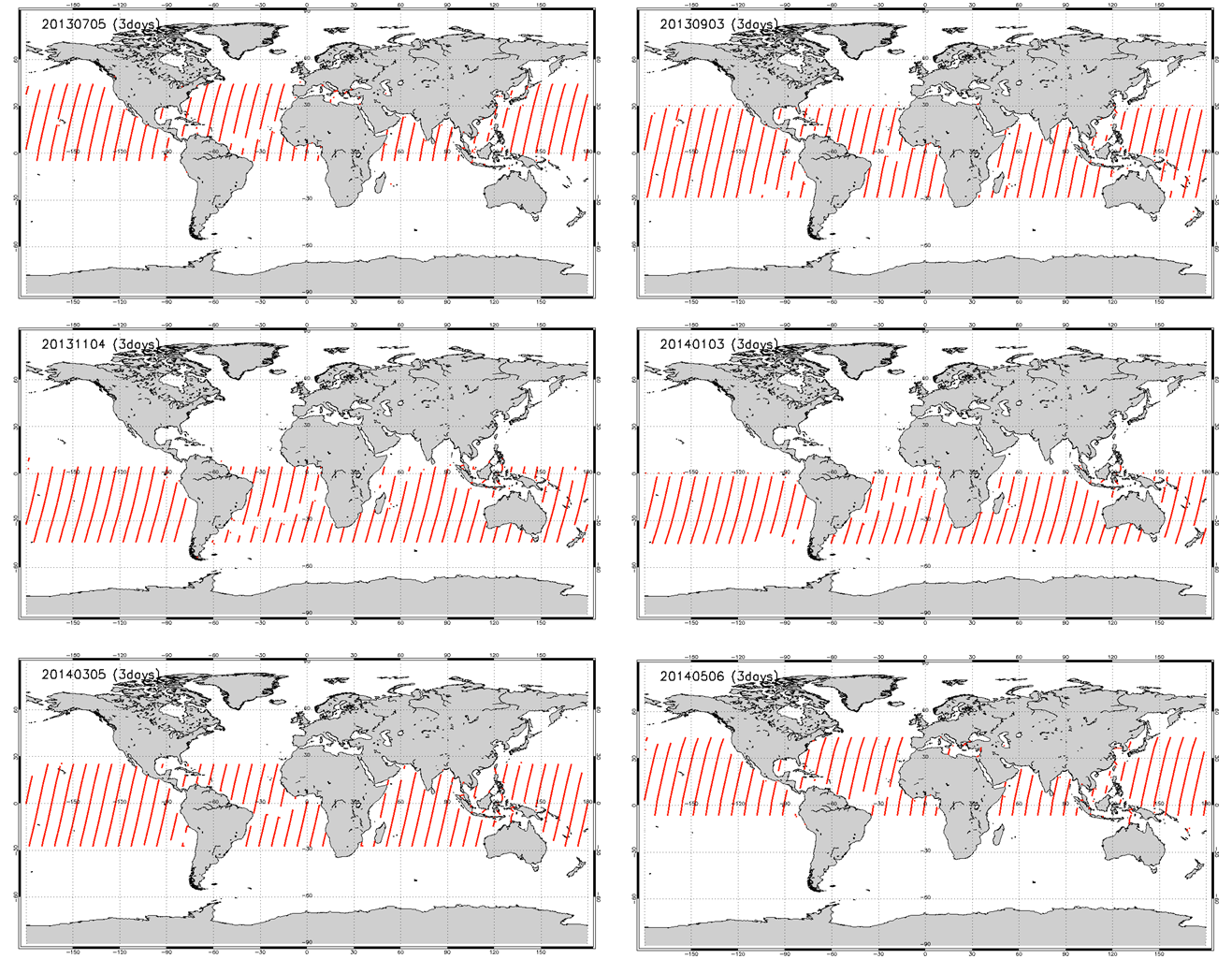
In order to extend the area of glint observation, glint observation points are determined with the summer and the winter geometries where the inclination of the earth's axis towards the sun becomes maximum, and are fixed throughout the year. The latitude range for glint observation was further extended three times in increments of 3 degrees on Sep. 10, 2014, Jun. 2, 2015, and Jan. 5, 2016 (, by not only tracking the exact specular points but also tracking along the principal plane of the specular reflection).
Example of 3-day glint observation points before May 6, 2013. Different glint observation plans were used for different seasons.
Example of 3-day glint observation points after May 6, 2013. A common glint observation plan was used throughout the year.
Incremental extension of the glint observation coverage. Each map shows an example of 3-day glint observation points for different latitude limits; upper-left: before extensions, upper-right: after 1st extension on Sep. 10, 2014, lower-left: after 2nd extension on Jun. 2, 2015, lower-right: after 3rd extension on Jan. 5, 2016.
